Missing data and multiple imputation in clinical epidemiological research

(1)

Clinical Epidemiology

Dove

press

M E T H O D O L O G Y

open access to scientific and medical research

Open Access Full Text Article

Missing data and multiple imputation in

clinical epidemiological research

Alma B Pedersen1

Ellen M Mikkelsen1

Deirdre Cronin-Fenton1

Nickolaj R Kristensen1

Tra My Pham2

Lars Pedersen1

Irene Petersen1,2

1_{Department of Clinical Epidemiology,} Aarhus University Hospital, Aarhus N, Denmark; 2_{Department of} Primary Care and Population Health, University College London, London, UK

Abstract: Missing data are ubiquitous in clinical epidemiological research. Individuals with missing data may differ from those with no missing data in terms of the outcome of interest and prognosis in general. Missing data are often categorized into the following three types: missing completely at random (MCAR), missing at random (MAR), and missing not at random (MNAR). In clinical epidemiological research, missing data are seldom MCAR. Missing data can constitute considerable challenges in the analyses and interpretation of results and can potentially weaken the validity of results and conclusions. A number of methods have been developed for dealing with missing data. These include complete-case analyses, missing indicator method, single value imputation, and sensitivity analyses incorporating worst-case and best-case scenarios. If applied under the MCAR assumption, some of these methods can provide unbiased but often less precise estimates. Multiple imputation is an alternative method to deal with missing data, which accounts for the uncertainty associated with missing data. Multiple imputation is implemented in most statistical software under the MAR assumption and provides unbiased and valid estimates of associations based on information from the available data. The method affects not only the coefficient estimates for variables with missing data but also the estimates for other variables with no missing data.

Keywords:missing data, observational study, multiple imputation, MAR, MCAR, MNAR

Introduction

Despite implementation of standardized data collection forms, missing data are ubiquitous in clinical epidemiological research. Missing data occur in various data sources (databases, medical records, and patient reported data), study designs, data collection methods (paper-based and online registration forms), registration time (eg, pretreatment and posttreatment), and registration frequency (eg, one postoperative outcome measurement and several follow-up measurements). Missing data can occur for multiple reasons – loss to follow-up, failure to attend medical appointments, lack of measurements, failure to send or retrieve questionnaires, and inaccurate transfer of data from paper registration to an electronic database.1

Individuals with missing data may differ from those with complete data in terms of the outcome of interest and prognosis in general. For example, those who are healthier may be less likely to visit their doctor and hence less likely to have blood pressure recorded. Studies on self-reported data show that individuals who have missing data on one variable are often likely also to have missing data on other variables. Our previous research demonstrated that patients with missing data on smoking often have missing data on other lifestyle variables.2_{Missing data can constitute considerable challenges} Correspondence: Alma B Pedersen

Department of Clinical Epidemiology, Aarhus University Hospital, Olof Palmes Alle 43-45, 8200 Aarhus N, Denmark Email [email protected]

Journal name: Clinical Epidemiology Article Designation: METHODOLOGY Year: 2017

Volume: 9

Running head verso: Pedersen et al

Running head recto: Multiple imputation method DOI: http://dx.doi.org/10.2147/CLEP.S129785

Clinical Epidemiology downloaded from https://www.dovepress.com/ by 118.70.13.36 on 20-Aug-2020

For personal use only.

This article was published in the following Dove Press journal: Clinical Epidemiology

15 March 2017

(2)

Dovepress Pedersen et al

in the analyses and interpretation of results and potentially weaken the validity of results and conclusions.3_{Missing data}

are problematic because of the risk of bias, which depends on the type of missing data, the extent of the data that are miss-ing, and the way of dealing with missing data in the analyses.4

The overall aim of this paper is to provide clinical epide-miological researchers with insights on the missing data. The specific aims of this paper are to: 1) describe methods often used for dealing with missing data in the analytic phase and highlight their shortfalls; 2) introduce multiple imputation as an alternative method, highlighting its advantages over “traditional” methods; and 3) discuss reporting of the results from multiple imputation analyses.

Types of missing data

Missing data are often categorized into the following three types: missing completely at random (MCAR), missing at random (MAR), and missing not at random (MNAR).5,6

When individuals with missing data are a random subset of the study population, the probability of being missing is the same for all cases; missing data are denoted as MCAR.7_An

example of MCAR is when a glass slide with biopsy material from a patient is accidentally broken such that pathology and histology tests cannot be performed, or when individuals had no blood pressure measured as the equipment was broken. Thus, under MCAR, missing data do not depend on either observed data or unobserved data.

In contrast to MCAR, the term MAR is counterintuitive. MAR occurs when the missingness depends on information we have already observed.7_{For example, data in a}

depres-sion survey can be said to be MAR, given gender if men are less likely than women to fill out the survey. Once gender is accounted for, the missingness does not depend on the level of their depression. Another example of MAR is when, in a study of weight, data on weight are less likely to be recorded for younger individuals, because they do not attend health care facilities as often as older individuals.

When the probability that data are missing depends on the unobserved data, such as the value of the observation itself, then the missing data are denoted as MNAR.7_{For example,}

overweight or underweight individuals may be more likely to have their weight measured than individuals with normal weight, even after age is accounted for. Thus, the reason for missingness is related to unobserved characteristics of the individual, and thereby, data are MNAR. Another example is when individuals with severe depression, or adverse effects from antidepressant medication, are more or less likely to complete a survey on depression. A third example is when

data on income are missing, and the probability of missing-ness is related to the level of income, eg, those with very low or high income refuse to report their income.

For the most part, in clinical epidemiological research, miss-ing values are neither MCAR nor MNAR but MAR.7_Observed

data can give us some indication of whether missing data are MCAR,8_{but we are not able, from these data alone or simple}

test, to evaluate whether missing data are MAR or MNAR.7

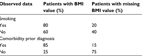
By tabulating the characteristics of individuals with missing data against those without, we can evaluate whether data are likely to be missing conditioning on these characteristics. We illustrate this in an example where a number of individuals are lacking body mass index (BMI) measurements (Table 1). In this example, we can see that among smokers, the proportion of individuals with BMI observed is higher compared to non-smokers. Similarly, among patients with known comorbidity prior surgery, the proportion of individuals with BMI observed is higher compared to that of those without known comorbidity. Thus, we can conclude that the data are not MCAR.

Graph theories have been helpful in a number of disci-plines in the fields of mathematics, engineering, computer science, and biology to determine or evaluate the mechanisms of missingness.9_{In epidemiological research, causal}

graphi-cal models, such as directed acyclic graphs (DAGs), can be used to determine whether data are MAR, MNAR or MCAR, thereby informing the most appropriate analytic method to deal with missing values.

Methods to minimize missing data

in the design phase

There are many ways to minimize the extent of missing data. It may be helpful to incorporate standardized rules to optimize data collection, such as training staff to collect and coordinate data collection, using well-defined data defini-tions, and incorporating logic and range checks for each data element. Pilot studies can help to identify variables particularly susceptible to missing values, and steps can be

Table 1An example of a situation when data are MAR rather than MCAR

Observed data Patients with BMI value (%)

Patients with missing BMI value (%) Smoking

Yes 80 20

No 60 40

Comorbidity prior diagnosis

Yes 85 15

No 25 75

Abbreviations: BMI, body mass index; MAR, missing at random; MCAR, missing completely at random.

(3)

Dovepress Multiple imputation method

taken to improve completeness.10_{Regular monitoring of}

data quality and completeness provides essential feedback to clinicians and researchers on the extent of missing data.11

Furthermore, when collecting information about the quality of life or other sensitive issues, patients may be asked to provide reasons for refusing to participate, such as a lack of time, problems understanding language, or lengthy or too intimate questionnaires. This information can be used in the analyses of data and interpretation of the results.

Methods of dealing with missing

data in the analytic phase

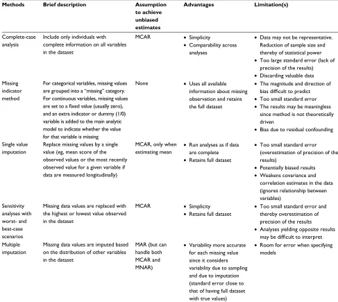
Several statistical approaches have been developed for dealing with missing data (Table 2). The most common

methods can be classified into one of the following groups: 1) complete-case analyses, 2) missing indicator method, 3) single value imputation, and 4) sensitivity analyses incor-porating worst-case and best-case scenarios. An alternative method of dealing with missing data in the analytic phase is multiple imputation.12,13_{Alternatives to multiple imputation}

include likelihood-based approach and probability weight-ing;3_{however, they are not the focus of this paper.}

Complete-case analysis

Complete-case analysis is the most widely used method to deal with missing data.13_{This method, also known as}

“list-wise deletion”, involves excluding individuals with missing data from the analyses. It is popular because it is easy to

Table 2 Proposed methods for dealing with missing data in the analytic phase

Methods Brief description Assumption

to achieve unbiased estimates

Advantages Limitation(s)

Complete-case analysis

Include only individuals with complete information on all variables in the dataset

MCAR • Simplicity

• Comparability across analyses

• Data may not be representative. Reduction of sample size and thereby of statistical power

• Too large standard error (lack of precision of the results)

• Discarding valuable data Missing

indicator method

For categorical variables, missing values are grouped into a “missing” category. For continuous variables, missing values

are set to a fixed value (usually zero),

and an extra indicator or dummy (1/0) variable is added to the main analytic model to indicate whether the value for that variable is missing

None • Uses all available information about missing observation and retains the full dataset

• The magnitude and direction of

bias difficult to predict

• Too small standard error

• The results may be meaningless since method is not theoretically driven

• Bias due to residual confounding

Single value imputation

Replace missing values by a single value (eg, mean score of the observed values or the most recently observed value for a given variable if data are measured longitudinally)

MCAR, only when estimating mean •

Run analyses as if data are complete

• Retains full dataset

• Too small standard error (overestimation of precision of the results)

• Potentially biased results

• Weakens covariance and correlation estimates in the data (ignores relationship between variables)

Sensitivity analyses with worst- and best-case scenarios

Missing data values are replaced with the highest or lowest value observed in the dataset

MCAR • Simplicity

• Retains full dataset

• Too small standard error and thereby overestimation of precision of the results

• Analyses yielding opposite results

may be difficult to interpret

Multiple imputation

Missing data values are imputed based on the distribution of other variables in the dataset

MAR (but can handle both MCAR and MNAR)

• Variability more accurate for each missing value since it considers variability due to sampling and due to imputation (standard error close to that of having full dataset with true values)

• Room for error when specifying models

(4)

implement and it is the default option in most statistical packages. However, the results of such analyses may yield biased estimates of associations, because complete cases are assumed to be a random sample of the whole population, ie, data are MCAR. That is not always the case, as often individu-als with complete data are different from those with missing data, and missingness can depend on either observed data or unobserved data. By comparing data in a UK Primary Care Database with a population survey, Marston et al1_showed

that the distributions of alcohol consumptions and smoking were different in the two data sources. This may suggest that data in these two variables are not MCAR. Complete-case analyses in this case may have serious consequences if the aim of a future study is to investigate an association between alcohol and postoperative complications. Another issue with complete-case analysis is that a large proportion of valuable research data are discarded, which affects the statistical power and precision of the estimates. In some cases, it may be rea-sonable to use complete-case analyses, such as when working with large datasets with few missing observations, because the risk of bias is minimal and the precision is still good.14

Missing indicator method

Under the missing indicator method, missing values are not imputed. Instead, for incomplete categorical variable(s), missing data are grouped into an additional “missing” egory; in the aforementioned example, BMI could be cat-egorized as underweight (BMI <18.5 kg/m2_{), normal (BMI}

18.6–24.9 kg/m2_{), overweight (BMI 25–29.9 kg/m}2_{), obese}

(BMI ≥30 kg/m2_{), and missing. For incomplete continuous}

variables, missing values are set to a fixed value (usually

zero), and an extra indicator or dummy (1/0) variable is added to the main analytic model to indicate whether the value for that variable is missing. The method is popular because it retains the full dataset where no observations are excluded. However, even under the MCAR assumption and with very few missing observations, this method is still subject to bias.12_{If the method is used for missing data on potential}

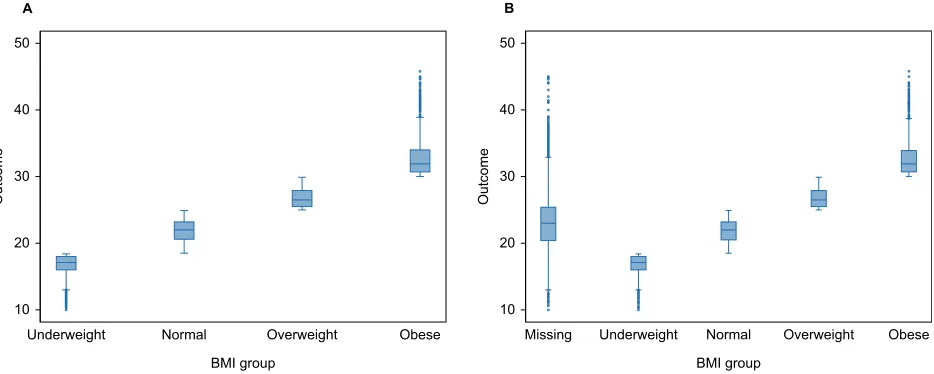
confounder variables, the estimates will be biased due to residual confounding. Figure 1 illustrates an example of a linear relationship between BMI categories and the outcome in a full dataset (on the left) and how the inclusion of a miss-ing BMI data category biases the relationship between BMI and the outcome (on the right).

Single value imputation

Under single value imputation, missing data are replaced by a single value, such as the mean score of the complete cases in the study sample (ie, mean imputation).13_{For example,}

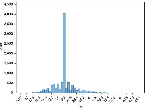
missing BMI values can be replaced with the sample mean BMI value calculated from individuals with observed BMI (Figures 2 and 3). Figures 2 and 3 illustrate normally uted BMI values in a full dataset and how normally distrib-uted data can be distorted in a dataset where 35% missing BMI values are replaced with the observed mean BMI value. In longitudinal studies where some variables are measured repeatedly, for example, yearly controls of glycated hemoglo-bin (HbA1c), the “last observation carried forward” approach can be used where missing values are replaced with the most recently observed value for a given variable. Another single imputation approach is regression-based single imputation of missing values (also known as predicted mean imputation), in

Figure 1 Distribution of BMI values by outcome in full dataset (A) and in a dataset with 35% missing values (B) for BMI handled by creating a missing BMI category.

Abbreviation: BMI, body mass index.

A

10 20 30 40 50

Outcom

e

Underweight Normal Overweight Obese

BMI group

B

10 20 30 40 50

Outcom

e

Missing Underweight Normal Overweight Obese

BMI group

(5)

which values of the missing observations are predicted using a regression model based on the complete cases.

In general, single imputation methods do not account for the uncertainty of missing data, and as a result, standard errors of the estimates are likely to be too small (thereby overestimating the precision of the results). This can poten-tially lead to Type 1 error (ie, identifying an association when none exists).12_{Mean imputation also does not preserve the}

relationships between variables; it only preserves the mean of the observed data. Therefore, if the data are MCAR, the estimate of the mean remains unbiased.4,12_{Under MCAR,}

if our aim is to estimate means (which is rarely the main focus of research studies), mean imputation will not bias the estimates; it will only bias the standard errors as mentioned previously. Since most of the research studies are interested in the relationship between variables and not just the mean,

mean imputation should be avoided in general. It has been pointed out previously that last observation carried forward method can produce biased estimates in both directions even under MCAR and have warned against using this method as the first or only choice for handling missing data.3

Sensitivity analyses with worst-case

and best-case scenarios

This method involves the replacement of missing values with the worst or best value in the observed data.15_{For example,}

analyses can be performed by replacing missing data with the highest or lowest observed value and running regression models afterward in order to examine the association of inter-est. The results of these two regression analyses can then be compared. When both analyses produce similar estimates of an association, it is rather straightforward to draw conclu-sions about the effect of missing data. However, analyses yielding opposing results can be difficult to interpret. If we have information on exposure but lack outcome data on some patients, we can replace missing data with the worst case (eg, death at the end of follow-up) or best case (patient is alive at the end of follow-up) and compare the results afterward. The usual procedure in smoking cessation studies is to assume that nonrespondents (missing smoking data) have resumed smoking.16_{Thus, the data are analyzed as if all}

nonrespon-dents have returned to active smoking, which might not be a correct assumption. Barnes et al16_{showed in a simulation}

study that this method yields biased estimates.

Multiple imputation

Multiple imputation4,5,17_{solves the problem of “too small or}

too large” standard errors obtained using traditional methods of dealing with missing data presented in Table 2. The aim of multiple imputation is to provide unbiased and valid estimates of associations based on information from the available data ie, yielding estimates similar to those calculated from full data.3

Missing data and hence multiple imputation may affect not only the coefficient estimates for variables with missing data but also the estimates for other variables with no missing data.

Multiple imputation is widely recognized as the standard method to deal with missing data in many areas of research, and the method has become more popular with the increas-ing availability of software. A full description of multiple imputation is beyond the scope of this paper, but we provide a brief overview of its assumptions, implementation, and meth-odologies. More detailed description of the statistical theory of multiple imputation is provided by Rubin,18_{Carpenter and}

Kenward,19_{and Buuren.}3 Figure 2 Normal distribution of observed BMI in a full dataset of 10,000

observations.

0 500 1,000 1,500 2,000 2,500 3,000 3,500 4,000 4,500

Count

10.2 12 13.8 15.6 17.419.2 21 22.824.6 26.4 28.2 3031.8 33.6 35.437.2 3940.8 42.644.4

BMI

Figure 3 Distribution of BMI in a dataset of 10,000 observations, where 35% of BMI values are missing and replaced by the observed mean BMI value.

0 500 1,000 1,500 2,000 2,500 3,000 3,500 4,000 4,500

Coun

t

10.2 12 13.8 15.6 17.419.2 2122.824.626.428.2 3031.833.635.4 37.2 3940.8 42.6 44.4

BMI

(6)

The multiple imputation procedure in most statistical software builds on the MAR assumption,20_{but the method}

can handle both MCAR and MNAR.3_{Although we cannot}

prove whether data are MAR, it is likely that in many situ-ations, the MAR assumption is more plausible when more variables are included in the multiple imputation model.21,22

Stages to implement multiple

imputation

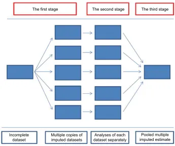
A statistical analysis using multiple imputation typically comprises of three major stages.

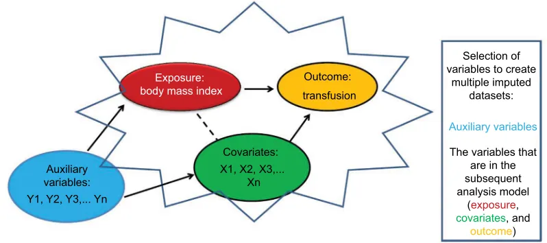
In the first stage, we select independent variables that may help to impute variables with missing data (Figure 4). This should include all variables that are in the subsequent analysis model (exposures, covariates, and outcome). In addi-tion, we may want to include variables that help make the MAR assumption plausible; the so-called auxiliary variables. Including these variables may reduce bias and improve the precision of the estimates.

Then, we create multiple imputed datasets where the indi-vidual data may vary between datasets (Figure 5). Missing values in each dataset are drawn from the distribution of the missing data given in the observed data.18_{As an example, the imputed}

values generated in the five imputed datasets for BMI are listed in Table 3. The table shows a variation of imputed values between imputed datasets and also between patients, reflecting the fact that we will never know what the “true” value was.

In the second stage, the association of interest is estimated in each of the imputed datasets using the chosen statistical method (eg, logistic regression) (Figure 5). Thus, coeffi-cient estimates with corresponding standard errors can be

calculated as a measure of association in each imputed dataset. There is variability both within and between the imputed datasets because of the uncertainty related to missing values.18

In the third stage, measures of association from each imputed dataset are combined by Rubin’s rules, with the corresponding standard errors (and hence the confidence intervals [CIs]) accounting for both the between- and within-imputation variations (Figure 5).19,23

Multiple imputation algorithms are implemented in all major statistical software (eg, SPSS, Stata, SAS, and R), which contain many detailed examples and step-by-step tutorials on both univariate and multivariate multiple imputations.3,24,25

Further considerations

Which variables should be included in the multiple imputa-tion model?

As we emphasize earlier, all variables used in the subse-quent analytic model need to be included in the imputation model (Figure 4). In addition, we can increase the precision and minimize the bias by including auxiliary variables in the imputation model. For auxiliary variables to have an impact, they would need to fulfill one of following criteria: 1) the auxiliary variable should be associated with the values of the incomplete variables, and 2) the auxiliary variable should be associated with the value of the incomplete variables and the likelihood of the data being missing. Auxiliary variables that are strongly associated with both the value and the miss-ingness are more likely to have an impact on the results of multiple imputation and reduce bias.19_{Based on our}

knowl-edge of the data, research question, or literature, we may

Figure 4 Selection of variables in order to create multiple imputed datasets when looking into the association between body mass index and transfusion risk. Exposure:

body mass index

Auxiliary variables:

Outcome: transfusion

Selection of variables to create

multiple imputed datasets:

Auxiliary variables

The variables that are in the subsequent analysis model

(exposure,

covariates, and

outcome) Covariates:

Y1, Y2, Y3,... Yn

X1, X2, X3,... Xn

(7)

a priori know that several variables we believe make good auxiliary variables. If we are not sure, these relationships can be identified by setting up, 1) a logistic regression model with the missingness (as 0 or 1) being the outcome and auxiliary variables being the explanatory variables, or 2) a regression model with the incomplete variable as the outcome and aux-iliary variables again as explanatory variables. In situations with many variables, multiple outcomes of interest, or large data sets, White et al23_{suggested to run a small number of}

imputations (also one single imputation) and then explore the associations within that dataset and select variables. In some cases, multiple imputation may provide similar results to complete-case analysis, but we will not know beforehand. The similarity can occur due to the lack of predictive covari-ates in the imputation model.

How many imputed data sets?

Traditionally, it has been suggested that three to five imputed datasets are sufficient.3,26_{The argument was that even with}

50% missing information, five imputed data sets would pro-duce point estimates that are 91% as efficient as those based on an infinite number of imputations.26_{However, Graham}

et al27_{showed that the statistical power and precision of}

estimates can be improved by creating many more imputed datasets depending on the amount of missing information and the tolerance for the loss of power. Later, Bodner28

and White et al23_{suggested the rule of thumb in order to}

increase a level of reproducibility of the results in practice; the number of imputations should be similar to the percent-age of incomplete cases. Buuren3_{suggested a compromise}

solution, using five imputations for model building in the

Figure 5 The three main stages of implementing multiple imputation. The first stage

Incomplete

dataset Multiple copies ofimputed datasets dataset separatelyAnalyses of each imputed estimatePooled multiple The second stage The third stage

Table 3 An example of the imputed missing BMI values generated with five imputed datasets

Patient number

Imputed data set 1 (BMI 1)

10 25.3 26.4 27.0 24.8 29.7

25 19.7 21.3 22.3 20.5 23.8

23 22.1 27.6 22.9 28.1 25.8

150 20.1 22.5 23.4 21.7 23.0

175 19.7 20.2 21.2 22.4 21.9

(8)

initial phase and increasing the number of imputations to the average percentage of missing data in the final phase of the analyses.

Reporting the results of multiple imputation analyses

After reviewing 59 papers from the general medical journals from 2002 to 2007 using multiple imputations, Sterne et al4

suggested guidelines for reporting such analyses, extending the Strengthening the Reporting of Observational Studies in Epidemiology (STROBE)guidelines.29_{The guidelines}

sug-gest reporting the results of both complete-case and multiple imputation methods, if possible, and particularly where there are differences in the results. Furthermore, the guidelines suggest to report the extent of missing data, the reasons for missingness, the assumptions for the multiple imputation model, and the number of imputed datasets and to specify the variables included in the multiple imputation model.

Multiple imputation example

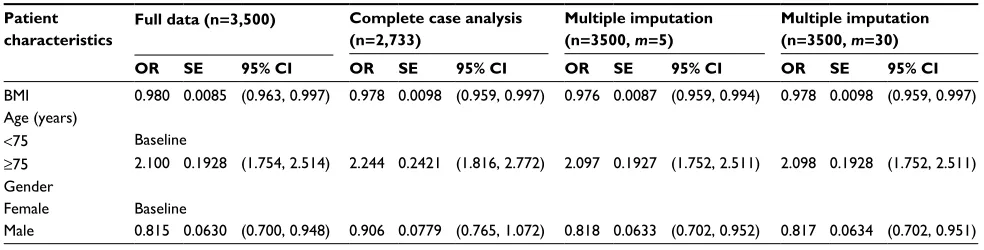
In this example, we evaluated the performances of complete-case analysis and multiple imputation and presented results in Table 4. This example, which resembles the association between the risk of blood transfusion within 7 days of hip fracture surgery in elderly patients and their BMI level at admission to the hospital, uses a dataset of 3,500 patients with no missing data. The model of interest is a logistic regression model of the odds of having blood transfusion (binary out-come – no/yes) conditional on patients’ BMI level (continuous exposure), adjusted for patients’ gender (binary variable – female/male), and age (binary variable – <75 or ≥75 years).

First, the model of interest is fitted to this dataset, referred to as “full data”, and parameter estimates (odds ratios) and associated 95% CIs and standard errors are recorded. Second, data in BMI are made MAR conditional on the outcome,

gender, and age, using a missingness mechanism, which results in 767 patients (22%) with missing BMI values. Miss-ing data in BMI are then handled usMiss-ing complete-case analysis and multiple imputation, and parameter estimates and associ-ated standard errors are also recorded and compared with the full data results. Multiple imputation is performed using m=5 and m=30 imputed dataset, and the imputation model for BMI includes all variables in the model of interest (outcome, age, and gender). Odds ratio estimate for BMI under complete-case analysis is similar to the corresponding value in the full data (0.978 and 0.980, respectively), with comparable standard errors (0.0098 and 0.0085, respectively). Multiple imputation using 5 and 30 imputations produced similar results for BMI. Parameter estimates for other variables under complete-case analysis are biased in comparison to full-observed data, with generally higher standard errors. While the significance of gender is detected in the full-observed data and multiple imputation, the effect of gender is apparently disguised by the missing data in complete cases due to the large bias in point estimate, which leads to Type 2 error. Overall, multiple imputation produces unbiased estimates and correct standard errors under the MAR assumption of BMI.

Conclusion

This paper provides insights on the type of missing data, traditional methods, and multiple imputation as alternative methods to deal with missing data, including their shortfalls and advantages.

• Missing data are ubiquitous to clinical epidemiological research.

• Missing data are often categorized into the following three types: MCAR, MAR, and MNAR. For the most part, in clinical epidemiologic research, missing values are neither MCAR nor MNAR but MAR.

Table 4 Association between BMI and risk of blood transfusion adjusted for age and gender

Patient characteristics

Full data (n=3,500) Complete case analysis (n=2,733)

Multiple imputation (n=3500, m=5)

Multiple imputation (n=3500, m=30)

OR SE 95% CI OR SE 95% CI OR SE 95% CI OR SE 95% CI

BMI 0.980 0.0085 (0.963, 0.997) 0.978 0.0098 (0.959, 0.997) 0.976 0.0087 (0.959, 0.994) 0.978 0.0098 (0.959, 0.997) Age (years)

<75 Baseline

≥75 2.100 0.1928 (1.754, 2.514) 2.244 0.2421 (1.816, 2.772) 2.097 0.1927 (1.752, 2.511) 2.098 0.1928 (1.752, 2.511) Gender

Female Baseline

Male 0.815 0.0630 (0.700, 0.948) 0.906 0.0779 (0.765, 1.072) 0.818 0.0633 (0.702, 0.952) 0.817 0.0634 (0.702, 0.951)

Note: Results are presented for full-observed data, complete-case analysis, and multiple imputation and contain point estimates for ORs, SEs, and 95% CIs.

Abbreviations: BMI, body mass index; CI, confidence interval; OR, odds ratio; SE, standard error.

(9)

• Missing data can constitute considerable challenges in the analyses and interpretation of results and can potentially weaken the validity of results and conclusion.

• Several methods have been developed for dealing with missing data including complete-case analyses, missing indicator method, single value imputation, and sensitivity analyses incorporating worst- and best-case scenarios. If applied under the MCAR assumption, these methods can provide unbiased estimates. If MCAR is not fulfilled, estimates may be biased. In addition, these methods are characterized by too large standard errors due to the lack of precision of the results or by too small standard errors due to the overestimation of the precision of results.

• Multiple imputation is an advanced method to deal with missing data. Standard imputation programs build on the MAR assumption, but the method can handle both MCAR and MNAR, although imputation is considerably more com-plex under MNAR. Multiple imputation provides unbiased and valid estimates of associations based on information from the available data – ie, yielding estimates similar to those calculated from full data. The method affects not only the coefficient estimates for variables with missing data but also the estimates for other variables with no missing data.

• In order to increase the transparency and understanding of the research results, we recommend the use of extended STROBE guidelines for reporting of multiple imputation analyses.

Author contributions

All authors contributed to the conception of the study, study design, and the discussion and interpretation of the results. ABP drafted and revised the article. All authors contributed to the manuscript for intellectual content and to drafting and critically revising the paper, gave final approval of the version to be published, and agree to be accountable for all aspects of the work.

Disclosure

The authors report no conflicts of interest in this work.

References

1. Marston L, Carpenter JR, Walters KR, Morris RW, Nazareth I, Petersen I. Issues in multiple imputation of missing data for large general practice clinical databases. Pharmacoepidemiol Drug Saf. 2010;19(6):618–626. 2. Pedersen AB, Baggesen LM, Ehrenstein V, Pedersen L, Lasgaard M,

Mikkelsen EM. Perceived stress and risk of any osteoporotic fracture. Osteoporos Int. 2016;27(6):2035–2045.

3. Buuren Sv. Flexible Imputation of Missing Data. Interdisciplinary Statistics Series. Boca Raton, FL: Chapman & Hall/CRC; 2012. 4. Sterne JA, White IR, Carlin JB, et al. Multiple imputation for missing

data in epidemiological and clinical research: potential and pitfalls. BMJ. 2009;338:b2393.

5. Graham JW. Missing data analysis: making it work in the real world. Annu Rev Psychol. 2009;60:549–576.

6. Rubin DB. Inference and missing data. Biometrika. 1976;63(3):581–592. 7. Donders AR, van der Heijden GJ, Stijnen T, Moons KG. Review: a

gentle introduction to imputation of missing values. J Clin Epidemiol. 2006;59(10):1087–1091.

8. Little RJA. A test of missing completelly at random for multivariate data with missing values. J Am Stat Assoc. 1988;83(404):1198–1202. 9. Mohan K, Pearl J, Tian J. Graphical models for inference with miss-ing data. In: Burges CJC, Bottou L, Wellmiss-ing M, Ghahramani Z, Weinberger KQ, editors. Advances in Neural Information Processing System 26 (NIPS-2013). Red Hook, NY: Curran Associates, Inc.; 2013:1277–1285.

10. Cappelleri JC, Zou KH, Bushmakin A, Alvir MJM, Symonds T. Patient-Reported Outcomes: Measurement, Implementation and Interpretation. Boca Raton, FL: CRC Press; 2013:2013.

11. Wisniewski SR, Leon AC, Otto MW, Trivedi MH. Prevention of missing data in clinical research studies. Biol Psychiatry. 2006;59(11):997–1000. 12. Greenland S, Finkle WD. A critical look at methods for handling miss-ing covariates in epidemiologic regression analyses. Am J Epidemiol. 1995;142(12):1255–1264.

13. Little RJA. Regression with missing X’s: a review. J Am Stat Assoc. 1992;87(420):1227–1237.

14. Apold H, Meyer HE, Espehaug B, Nordsletten L, Havelin LI, Flugsrud GB. Weight gain and the risk of total hip replacement a population-based prospective cohort study of 265,725 individuals. Osteoarthritis Cartilage. 2011;19(7):809–815.

15. Pedersen AB, Sorensen HT, Mehnert F, Overgaard S, Johnsen SP. Risk factors for venous thromboembolism in patients undergoing total hip replacement and receiving routine thromboprophylaxis. J Bone Joint Surg Am. 2010;92-A(12):2156–2164.

16. Barnes SA, Larsen MD, Schroeder D, Hanson A, Decker PA. Missing data assumptions and methods in a smoking cessation study. Addiction. 2010;105(3):431–437.

17. Klebanoff MA, Cole SR. Use of multiple imputation in the epidemio-logic literature. Am J Epidemiol. 2008;168(4):355–357.

18. Rubin DB. Multiple imputation after 18+ years. J Am Stat Assoc. 1996; 91(434):473–489.

19. Carpenter J, Kenward M. Multiple Imputation and Its Application. New York, NY: John Wiley & Sons; 2013.

20. Schafer JL, Graham JW. Missing data: our view of the state of the art. Psychol Methods. 2002;7(2):147–177.

21. Collins LM, Schafer JL, Kam CM. A comparison of inclusive and restrictive strategies in modern missing data procedures. Psychol Methods. 2001;6(4):330–351.

22. Moons KG, Donders RA, Stijnen T, Harrell FE Jr. Using the outcome for imputation of missing predictor values was preferred. J Clin Epidemiol. 2006;59(10):1092–1101.

23. White IR, Royston P, Wood AM. Multiple imputation using chained equations: issues and guidance for practice. Stat Med. 2011;30(4): 377–399.

24. van Buuren S. Multiple imputation of discrete and continuous data by fully conditional specification. Stat Methods Med Res. 2007;16(3):219–242. 25. StataCorp. Stata: Release 13. Statistical Software. College Station, TX: StataCorp LP; 2013. Available from: https://www.stata.com/manuals13/ mi.pdf. Accessed December 1, 2016.

26. Rubin DB. Introduction in Multiple Imputation for Nonresponse in Surveys. Hoboken, NJ: John Wiley & Sons, Inc; 1987.

27. Graham JW, Olchowski AE, Gilreath TD. How many imputations are really needed? Some practical clarifications of multiple imputation theory. Prev Sci. 2007;8(3):206–213.

28. Bodner TE. What improves with increased missing data imputations? Struct Equ Modeling. 2008;15(4):651–675.

29. von Elm E, Altman DG, Egger M, Pocock SJ, Gotzsche PC, Vanden-broucke JP; STROBE Initiative. The strengthening the reporting of observational studies in epidemiology (STROBE) statement: guide-lines for reporting observational studies. Lancet. 2007;370(9596): 1453–1457.

(10)

Dovepress

Clinical Epidemiology

Publish your work in this journal

Submit your manuscript here: https://www.dovepress.com/clinical-epidemiology-journal Clinical Epidemiology is an international, peer-reviewed, open access, online journal focusing on disease and drug epidemiology, identifica-tion of risk factors and screening procedures to develop optimal pre-ventative initiatives and programs. Specific topics include: diagnosis, prognosis, treatment, screening, prevention, risk factor modification,

systematic reviews, risk and safety of medical interventions, epidemiol-ogy and biostatistical methods, and evaluation of guidelines, translational medicine, health policies and economic evaluations. The manuscript management system is completely online and includes a very quick and fair peer-review system, which is all easy to use.

Dove

press

Pedersen et al