Smart Meter Data-based Three-Stage Algorithm to Calculate Power and Energy Losses in Low Voltage Distribution Networks

Article

Smart Meter Data-based Three-Stage Algorithm to

Calculate Power and Energy Losses in Low Voltage

Distribution Networks

Gheorghe Grigoras 1,_{*, Bogdan-Constantin Neagu} 2

1 _{Department of Power Engineering; “Gheorghe Asachi” Technical University of Iasi, Romania,}

[email protected];[email protected] (G.G.)

2 _{Department of Power Engineering; “Gheorghe Asachi” Technical University of Iasi, Romania}

[email protected] (B.C.N.)

* Correspondence: [email protected];[email protected] Tel.: +04 0232 278683 (G.G.)

Abstract: In the paper, an improved smart meter data-based three-stage algorithm to calculate the power/energy losses in the three-phase networks with the voltage level below 0.4 kV (low voltage - LV) is presented. In the first stage, a loading function of input data was built having as main feature the working at the same time with files from the database of smart metering system (SMS) containing the hourly electricity records, and files including the characteristic load profiles established by the Distribution Network Operator (DNO) for the consumers with standard energy meters depending the following factors: consumption class, day and season. In the second stage, a function which is based on the work with the structure vectors was implemented to identify easy the configuration of analysed networks. In the third stage, an improved version of forward/backward sweep-based algorithm was proposed to calculate fast the power/energy losses to three-phase LV distribution networks in balanced and unbalanced regime. A real LV rural distribution network from a pilot zone belonging to a Distribution Network Operator (DNO) from Romania was used to confirm the accuracy of the proposed approach. The comparison with the results obtained using the DigSilent PowerFactory Simulation Package certified the performance of the algorithm, the mean absolute percentage error (MAPE) being 0.94%.

Keywords: distribution networks; energy losses; three-stage algorithm; smart meters; characteristic load profiles

1. Introduction

Until a few years ago, the electric distribution networks were generally characterized by the lack of technical possibilities represented by smart devices that can help the Distribution Networks Operators (DNOs) in the supervisory, control and decision making processes. Although the low voltage (LV) distribution networks feed a high number of consumers, few information could have been gathered from inside (from the consumers and producers), with a delayed response time. In order to obtain as much data from the network, it is necessary to be installed smart meters which would allow the storage of supervised data (energy consumptions, active and reactive powers, voltages, power factors, harmonics etc.) and their transmission to the DNOs level.

The Smart Metering technology is essential for achieving the targets regarding the energy efficiency and renewable energy set for 2020, as well as the delineation of future smart grids. The introduction of smart metering system (SMS) in the European countries is finished in some countries and is in different stages in others [1-5]. Thus, a special attention should be paid to the management of databases built with the help of information provided by smart meters from consumers and producers for improving the energy efficiency in the low voltage networks. The benefits of smart

meters consist in the fact that, in addition to the metering function, they also provide a whole range of applications, such as the following [6, 7]:

• secure transmission of data to the consumer or a third party (for example Metering Operator), respectively to the DNO;

• bidirectional communication between the smart meters installed at consumer/prosumer sites and the concentrators (information management points) belonging to the DNO;

• remotely controlled connection/disconnection from the grid or demand limitation at consumer sites;

• implementing of differentiated time-of-use tariffs.

In these circumstances, the DNOs can get accurate online information regarding energy consumptions and productions from renewable sources, which allows them to calculate the energy losses and then to take some measures which will enable the low voltage networks to operate more energy efficient and better plan their investments. For the LV electrical networks, the information needed to calculate the power and energy losses is easy obtained if consumers are integrated into the SMS. In this context, the Decision-Maker should use accurate methods and to take into account all components (lines and transformers) to have a correct evaluation regarding the efficiency of own LV distribution networks. Thus, an accurate analysis of the steady-state corresponding the LV distribution network can be made through a real-time monitoring by means of the smart meters. Based on the obtained data, the following state variables could be immediately determined: the current flows on each line section, the voltage level in the nodes, and the power and energy losses on the all network elements and on the whole network.

More methods are presented in the literature to estimate the power/energy losses, but unfortunately, the loss factor formulas represents the support of them. For example, the statistical data determined from the active power profiles (the average value and the standard deviation) were used in [8] to calculate the loss factor in order to estimate the energy losses. A similar approach based on the average value and variation limits of the required power by consumers extracted from the active power profiles was proposed in [9]. The load profile and some primary variables of medium voltage (MV) feeders which refer at the length, loading factor at the peak load, and the distribution function of load have constituted the used data in [10] for the simulation studies in order to determine the repartition functions of power losses at the maximum loading. The difference between the incoming and outgoing energy amounts represents another approach presented in [11] to evaluate the energy losses in the distribution network. Also, the loss factors were calculated in [12] and [13] to evaluate the energy losses in distribution networks. A scaling factor was used in [14-16] for the characteristic load profiles with attached pseudo measurements performed in the balanced LV grids with distributed generation sources to estimate the power losses. In [17,18], the power losses computation used the loss factor and the load profile. The drawback of this method are the estimation of the two coefficients A and B as constants for given homogeneous loads or load profile. Moreover, in [19,20] the active power losses for three balanced (neglecting the neutral) LV feeders from a microgrid were calculated. All the aforementioned methods uses for Joule power losses estimation a simplified methodology based on Kirchhoff laws.

In relation to the approaches presented in the literature, the proposed algorithm has the following advantages identified in each stage:

• Stage I is based on an access function which loads at the same time files from two different database: the database of the SMS including the load and production profiles for the integrated consumers and the database containing the characteristic load profiles (CLPs) which are assigned the consumers with standard energy meters (non-integrated in the SMS). The CLPs are divided considering the following features: type of consumers (residential, non-residential, commercial, and industrial), the class of electricity consumption, day type (weekend and working), and season type (springer, summer, autumn, winter).

• Stage 2 has implemented a recognition function of the network topology based on the two structure vectors.

• Stage 3 has integrated on the improved version of forward/backward sweep-based algorithm to calculate fast the power/energy losses to three-phase LV distribution networks in balanced and unbalanced regime. Regarding the forward/backward sweep-based algorithm, it was mainly used in the medium voltage distribution networks to calculate the balanced, symmetric steady-state regime [25-27], [30]. But, the proposed version was adapted to the LV distribution networks that most often operate in unbalanced regime due to the chaotic allocation of the single-phase consumers on the phases.

Our approach use real data about the active and reactive power for both consumers and small-scale sources integrated in the LV distribution networks. Another particularity refer at the power/energy losses computation using a modified branch and bound (forward backward sweep) method. A pilot LV distribution network from a rural area belonging to a DNO from Romania was chosen to demonstrate the performance of the proposed algorithm. A comparison with the results obtained using the DigSilent PowerFactory (DSPF) simulation package certified the accuracy of algorithm. Even if the DSPF is one of the most powerful package in simulations of the processes from the generation, transmission, and distribution levels, it presents some disadvantages represented by the introduction of network elements (lines, loads, buses) requiring a long time period depending by the size of network and the loading of load profiles which should have a certain format. Therefore, this software is especially recommended in the off-line analyses.

The structure of paper is organized as following: Section 2 reveals the stages of proposed algorithm, detailing the load profiling process used for the non-integrated consumers in the SMS, Section 3 presents the results obtained in the case of a LV network from a pilot rural zone of a DNO from Romania and a comparison with simulations made using DSPF package, and Section 4 highlights the conclusions and the future works.

2. Three-Stage Algorithm to calculate the power/energy losses

The steady-state regime calculations using the very well-known iterative methods (Seidel-Gauss or Newton-Raphson) can be difficult performed for the LV distribution networks in order to obtain the energy losses. This occurs due to the following particular features represented by: the ill-conditioning given by the radial topologies, resistance with high values and reactance with small values (depending by the cross-sections of conductors), often operate in unbalanced regime due to the chaotic allocation of the single-phase consumers on the phases.

Taking into account the above features, a different approach based on the three-Stage Algorithm to eliminate these drawbacks will be presented in the following:

• Stage 1. The input data for the consumers referring to the energy characteristics are read from the databases which contains for each consumer the load profiles (the consumer is integrated in the SMS) or the CLPs (the consumer is not integrated in the SMS) depending by the class of electricity consumption, day type (weekend and working), and season type (springer, summer, autumn, winter). Also, the production profiles of the generators from the network are loaded by the input algorithm.

• Stage 3. The power/energy losses are determined using an improved variant forward/backward sweep algorithm which can work both in the balanced and unbalanced regimes, with or without distributed generation.

2.1. The first stage

Whatever type of consumer (residential, commercial, or industrial), there is its own consumption pattern which can be identified based on a load profile representing the consumed active and/or reactive power in a time frame. But, the access at these data can be available only if the consumer is integrated in the SMS. In this regard, the vast majority of the DNOs from the UE countries implemented projects in pilot zones to identify the efficiency of the integration in the SMS of the consumers. The expected results should refer at the following [1]:

• The energy consumption is monitored on-line with benefits for both parts: the DNOs to implement the energy efficiency measures, and the consumers to establish their pricing mode in function by the energy consumption behaviour.

• The analysis of recorded data must lead to optimal strategies regarding the increase of energy efficiency in the LV distribution networks of the DNOs.

• Extended the processed data (as load type profiles) at the networks from same area, without SMS implementation, to analyse their operation regime.

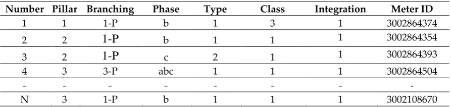
The algorithm accepts the input data using a similar format to the one available in the database of the DNOs. The records with the associated fields from the input file are indicated in Table 1.

Table 1. The format of input data

Number Pillar Branching Phase Type Class Integration Meter ID

1 1 1-P b 1 3 1 3002864374

2 2

1-P

3 2

1-P

4 3 3-P abc 1 1 1 3002864504

- - - -

N 3 1-P b 1 1 1 3002108670

Each field of a record will be detailed in the following:

• Number represents the allocated record for a certain consumer in the database of DNO.

• Pillar represents the identification number of each pillar made by the DNO for a rural LV distribution network. The pillars are numbered in all rural LV distribution networks to know where are connected the consumers. For example in Table 1, the consumer 1 is connected at the pillar 1, and the consumer 4 is connected at the pillar 3.

• Branching identifies the type of electric branching for each consumer: single-phase (1-P) or three-phases (3-P). These can be identified in the database with 1 (single-phase) or 3 (three-three-phases). • Phase allow to identify the phase(s) at which a consumer is allocated (if it is a 1-P consumer then

in the field the notations a, b, or c can be seen, and if it is a 3-P consumer then the notation abc can be observed).

• Type emphasizes if the consumer belongs the following consumption patterns: residential (ID is 1), non-residential, namely community buildings, hospitals, town halls, schools, etc. (ID is 2), commercial (ID is 3), and industrial (ID is 4).

• Integration allows the user to know if the meter is (value is equal with 1) or not (value is equal with 0) in the database of the SMS. If the meter is integrated, based on the ID of meter, the active and reactive power profiles of consumer can be loaded from the database. If a meter is not integrate then the daily energy indexes will be loaded from the database. In this last case, a CLP will be allocate the consumer using the algorithm presented in the next section in function by the records Type and Class. The associated active and reactive power profile will be finally obtained based on the loaded energy indexes.

A matrix will be loaded having a number of rows equal to the sampling size of active and reactive power profiles (quarter hour, half hour or one hour) and a number of columns with the size: 2 x 3 x total number of consumers. The signification of the 2 x 3 columns is given by the fact that for each consumer will be allocated three columns for active power and three columns for reactive power. Only columns associated to the connection phase of the consumers will have values different by 0 in the input matrix. Also, the algorithm can be used in the on-line calculations, the data being read as soon as they reached the data center.

2.1.1. Load Profiling Process based on Smart Meters Data

If a consumer is not integrated in the SMS, the DNO can assigned a CLP depending the different consumer’ types (residential, commercial and public), energy consumption class, and seasons (spring, summer, autumn and winter) which are obtained based on the processed data from the consumers with smart meter available [28, 29].

Thus, using the CLPs and the daily energy consumption for each consumer, without a smart meter implemented, the load profiles could be computed using the following algorithm. The deformalized load profile at consumer l is calculated with the relation:

(h) tc l (h)

l W CLP

P =  (1) where:

Pl(h)– the denormalized load profile at consumer l for each hour h = 1, …, 24, l = 1,…, Nc; tc – the type of the l-th consumer, l = 1,…, Nc;

CLPtc(h) – the characteristic load profile for the tc type of consumer (tc can be residential, non-residential, commercial or industrial), for each hour h = 1, …, 24;

Wl – the daily energy consumption for the consumer l;

Nc – total number of consumers without smart meter installed or with missing data in the SMS. Next, the denormalized profiles calculated above are adjusted by using the hourly values recorded by the smart meter from the electric substation, as follows:

24 ,..., 1 = =



P (2)

24 ,..., 1 = =



P (3)

ΔP(h)=Ptc(h)−Pm(h)−P_SM(h) h=1,...,24 (4)

24 ,..., 1 =               +  =



cor,l (5)

where:

Pm(h) - three-phase feeder measured load profile for the analysed period;

P(h)sm,n– active power measured with the smart meter at the consumer n, n = 1, …, NSM; NSM– total number of consumers integrated in the SMS.

2.2. The second stage

The topology of the analysed network will be very easy identified based on an algorithm which build two structure vectors (VS1 and VS2). The algorithm is explained hereinafter.

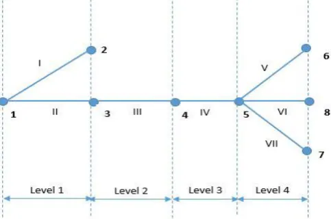
The process allows the clustering of each section at a hierarchical level, starting with the first section. To exemplify the procedure, a radial LV distribution network with 8 nodes (pillars) and 7 sections was considered (see Figure 1). The steps are described below for the network from Figure 1.

Figure 1. The topology of a radial LV distribution network

If it is adopted the following order to numbering the sections: 1-2 (I), 1-3 (II), 3-4 (III), 4-5 (IV), 5-6 (V), 5-8 (VI), and 5-7 (VII), then the size of the vector VS1 is equal with identified levels, and the elements represent the sections assigned at one certain level (1, 2, 3, or 4). The correlation between vectors VS1 and VS2 can be observed in Table 2, where the structure vectors are shown.

Table 2. The structure vectors for the LV distribution network from Figure 1

VS1 1 2 3 4

VS2 I

(1-2) II (1-3) III (3-4) IV (4-5) V (5-6) VI (5-8) VII (5-7)

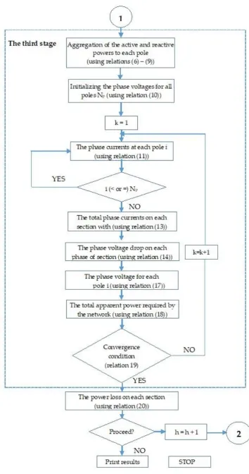
2.3. The third stage

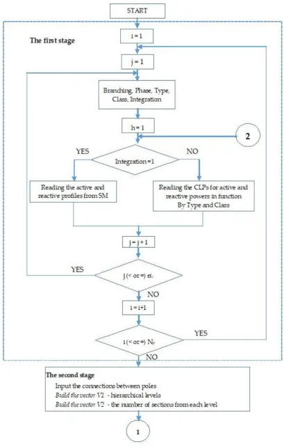
The calculations for the steady state regime from the each hour h, h = 1,…, H (in our case H = 24) will be made using an improved variant forward/backward sweep algorithm which can work both in the balanced and unbalanced regimes, with or without distributed generation. The following steps are taken to calculate the energy losses:

1. The loads from each node (pillar) are aggregated using for all consumers nic allocated at the pillar i, on the each phase {p} = {a, b, c} the data loaded from the database of the SMS or resulted from the profiling process:



P i = 1, …, Np, {p} = {a, b, c} (6)



Q i = 1, …, Np, {p} = {a, b, c} (7)

where Np represents the total number of pillars from the analysed networks.

If a generator is located in a node j (it can be at the same time and the consumer), connected at the pillar i then:

P{p}_j =P_c,i{p}_j −P_g,i{p}_j {p} = {a, b, c} (8)

i{p} j g, i{p} j c, {p} Q Q Q

where P_g,i{p}_j ,Qi{p}_g,j are the active and reactive power injected by the generator from the node j, connected at the pillar i, on the phases p = {a, b, c}, andP_c,i{p}_j ,Qi{p}_c,j are the active and reactive absorbed by node j.

2. The phase voltages are initialized at each node (pillar) from the distribution network with the recorded values on the LV side of electric substation (Us{p} ). The values could be different by the nominal voltage:

{p} s {

i U

U p}(0) = , i = 1, …, Np, i ≠ s , {p} = {a, b, c} (10)

3. Backward sweep:

3.1. The currents at the level of nodes (pillars) are calculated:

1) (k * {p} i * {p} i (k) {p} i U S I ₋      

= , k = 1, … Kmax, i = 1, …, Np, {p} = {a, b, c} (11)

{p} i {p} i {p}

i P j Q

S = +  (12) where k is the index of current iteration and Kmax expresses the maximum value of iterations introduced initially by the decision maker.

3.2. The current flow on each section (v-i) of the network are calculated:



v, I I

I , k = 1, … Kmax, i = 1, …, Np, {p} = {a, b, c} (13)

where: v is the pillar in up stream of pillar i; Next (i) is the set of pillars next to the pillar i; (v-i) is the section

4. Forward sweep:

4.1. The voltage drop on the phases {p} of all sections is calculated: (k) 0 i v, 0 i v, (k) {p} i v, i v, (k) {p} i

v, Z I Z I

ΔU =  +  , i = 1, …, Np, v ≠ i, {p} = {a, b, c} (14)

i v, i v, j X

R

Zv,i = +  (15)

where: Zv,i and Zv,i0 are the impedances of the phase {p} = {a, b, c} and neutral conductors (0); Iv,i0 represents the current which flows through the neutral conductor.

c i v, b i v, a i v, 0 i

v, I I I

I = + + (16) 4.2. The voltage on the phase {p} = {a, b, c} for each pillar i is calculated:

(k) {p} i v, (k) {p} v (k) {p}

i U ΔU

U = − , i = 1, …, Np, v ≠ i, {p} = {a, b, c} (17)

4.3. The total apparent power injected to the network is calculated:



S p} , {p} = {a, b, c} (18)

4.4. Testing the stopping condition of iterative process: s 1) (k {p} s (k) {p}

s S ε

S − −  , {p} = {a, b, c} (19)

where εS represents the imposed error by the decision maker to stop the iterative process. 5. If the iterative process is finished (the relation (19) is accomplished), the power loss on each section (v-i) is calculated:

2 (k) 0 i v, 0 i v, 2 (k) {p} i v, i v, (k) {p} i

v, R I R I

ΔP  + _ _

     

= , i = 1, …, Np, v ≠ i, {p} = {a, b, c} (20)

where Rv,i and Rv,i0 are the resistances of the phase and neutral conductors.

Figure 2.b. The flow-chart of algorithm (the third stage)

The proposed algorithm was tested on a real pilot LV electric distribution network belonging to a DNO from Romania. The topology of analysed network can be seen in Figure 3. The electric substation MV/LV supplies 3 distribution feeders.

Figure 3. The analysed LV distribution network

The three feeders have 189 pillars together. The pillars represent points where the consumers are connected using the single-phase (1-P) or three-phase (3-P) branching at the network, and these are identified through black circles. Each section has 40 meters, representing the distance between two pillars. The primary characteristics (number of pillars, total length, cable type, cable size, length of sections using given cable types, and number of consumers) are shown in Table 3. Also, consumers’ characteristics can be identified in Table 4.

Table 3. The characteristics of feeders

Feeder Length [m]

Conductor Type

Cross-section (phase+neutral)

[mm2]

Length [m]

r0 [Ω/km]

x0 [Ω/km]

Feeder 1 280 Classical 1x50+50 280 0.61 0.298

Feeder 2 3,880 Stranded 3x35+35 120 0.871 0.055 Classical 3x50+50 3,760 0.61 0.298

Feeder 3 3,520

Stranded 3x50+50 120 0.605 0.05 Classical 3x50+50 2,080 0.61 0.298 Classical 3x35+35 960 0.871 0.055 Classical 1x25+25 280 1.235 0.319 Classical 1x16+25 80 1.235 0.319

Total 7,680 Classical 7,440

Table 4. The characteristics of consumers

Consumers’ type 1-P 3-P

Phase a 83 -

Phase b 15 -

Phase c 100 -

Total 335 8

Consumption Class

[kWh/year]

0 – 400 150 5

400-1000 108 2

1000-2500 65 0

2500-3500 5 0

> 3500 7 1

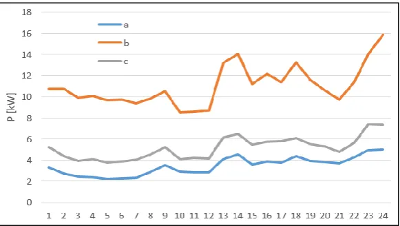
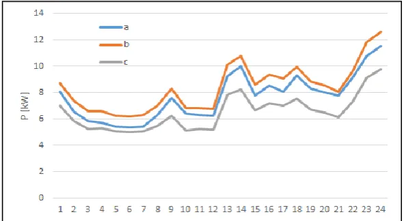
The details regarding the allocations at pillars and phases, and the type of consumers are indicated in Appendix A, Table A1. The connection phase of each consumer reflects the real situation, and this aspect helped to establish the true-to-reality unbalanced model. The hourly load records (active and reactive power profiles) for each consumer integrated in the SM system were imported from the database of the DNO for the day when the analysis was made. Based on these profiles, the phase loading at the LV level of electric substation was calculated for each feeder, see Figures 4, 5 and 6.

Figure 4. The phase loading on the first section of Feeder 1

Figure 6. The phase loading on the first section of Feeder 3

From Figure 4, it can be observed that all consumers from Feeder 1 are only allocated on the phase b. Feeder 2 has a high unbalance, the phase b is more loaded than the other two phases (a and c), see Figure 5. In this case, the current flow on the neutral conductor will lead at the high additional losses. For Feeder 3, the allocation of consumers on the phases of the feeder is more balanced, see Figure 6.

The steady-state regime calculations were performed at each hour h = 1, …, H (where H = 24). The total energy losses calculated with proposed algorithm for each feeder, on each phase and neutral conductor, on branching and main conductors are presented in Tables 5. The obtained results with the DSPF software are presented in Table 6 to emphasize the accuracy of proposed algorithm.

The detailed results obtained with proposed algorithm for each feeder are presented in Tables B1, B2, and B3 from Appendix B.

The absolute errors (ε) and percentage errors (δ) between both approaches, DSPF software and proposed algorithm (PA) are presented in Table 7, Figure 7, and Figure 8. The calculation relations are the following:

PA DSPF ΔW ΔW

ε= − , [kWh] (21)

100

ΔW ΔW ΔW

δ

DSPF PA

DSPF− _

= , [%] (22)

Table 5. The energy losses calculated with PA algorithm, [kWh]

Feeder Phase Neutral TOTAL

a b c

Ma

in

con

d

u

ct

or

s Feeder 1 0.000 0.047 0.000 0.058 0.105 Feeder 2 0.529 9.973 2.455 8.055 21.012

Feeder 3 6.370 5.411 5.726 1.586 19.092

TOTAL 6.900 15.430 8.180 9.699 40.209

Bra

n

ch

in

g

con

d

u

ct

or

s Feeder 1 0.000 0.006 0.000 0.004 0.010 Feeder 2 0.055 0.173 0.019 0.162 0.410

Feeder 3 0.072 0.052 0.052 0.086 0.263

TOTAL 0.127 0.232 0.072 0.253 0.682

Table 6. The energy losses calculated with DSPF software, [kWh]

Feeder Phase Neutral TOTAL

a b c

Ma

in

con

d

u

ct

or

s Feeder 1 0.000 0.043 0.000 0.054 0.097 Feeder 2 0.509 9.647 2.433 7.765 20.354

Feeder 3 6.099 5.438 6.184 1.572 19.293

TOTAL 6.608 15.129 8.616 9.391 39.744

Bra

n

ch

in

g

con

d

u

ct

or

s Feeder 1 0.000 0.006 0.000 0.004 0.010 Feeder 2 0.053 0.218 0.020 0.187 0.479

Feeder 3 0.069 0.055 0.059 0.090 0.273

TOTAL 0.122 0.279 0.079 0.281 0.762

TOTAL 6.731 15.408 8.696 9.671 40.506

Table 7. The values of energy losses and errors

Approach Phase Neutral Total a b c

PA [kWh] 7.03 15.66 8.25 9.95 40.89

DSPF [kWh] 6.73 15.41 8.70 9.67 40.51

ε

δ

From Table 7, it can be observed that the percentage errors of energy losses in conductors are in the range [1.62 – 5.17] and below 1 percent (0.94) for the total energy losses. Also, it can highlighted a high value of energy loses in the neutral conductor. These represent about 25 percent from the total energy losses which means that the DNO should take the balancing measures (especially in the case of Feeder 2).

Figure 8. The hourly energy losses computed with both approaches, [%]

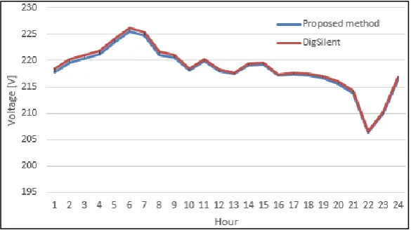
In terms of phase voltages, these were calculated for each pillar. The obtained values for the farthest pillars are represented in the Figures 9-11 (pillar P95 – Feeder 2) and Figures 12-14 (pillar P188 – Feeder 3).

Figure 9. The phase voltage (phase a) at Pillar P95 – Feeder 2

Figure 11. The phase voltage (phase c) at Pillar P95 – Feeder 2

Figure 12. The phase voltage (phase a) at Pillar P188 – Feeder 3

Figure 14. The phase voltage (phase c) at Pillar P188 – Feeder 3

The detailed results obtained with proposed algorithm for each pillar are presented in Table 4B from Appendix B.

An analyse of Figures 9 - 14 highlighted that at the pillar P95 the phase voltages are inside of admissible limits (nominal voltage ± 10 %), and at the pillar P188 only the voltage on the phase b is corresponding, but equal with minimum value (nominal voltage – 10 %). The voltages on the phases a and c are slightly below the minimum limit with 0.02 %. The nominal phase voltage in Romania is 230 V. Thus, the DNO should take the measures to improve the voltage level in this final node (tap changing of transformer from the electric substation).

The mean percentage errors (MPE) of the phase voltages are presented in Figures 15 and 16. These were calculate with the following relation:



=

−

= 24

1

t DSPF

PA DSPF ΔW

Δ ΔW

24 100

MPE , [%] (23)

It can be observed that the MPEs is below 0.3 % on each phase at both pillars (P95 and P188).

Figure 16. The MPE on the phase, Pillar P188

4. Conclusions

The paper presents an improved smart meter data-based three-stage algorithm to power/energy losses calculation in three-phase LV distribution networks. The three stages refer to: The first stage. The data files are loaded from the databases of the DNOs refers at the energy consumption of consumers taking into account if they are or not integrated in the SMS; The second stage. Identification of the topological structure base on the two vectors; and The third stage. The power/energy losses are calculated using an improved variant of the forward/backward sweep-based algorithm adapted to the three-phase LV distribution networks operating in the balanced and unbalanced regimes.

The obtained results considering a pilot distribution network belonging to a DNO from Romania with the consumers integrated in the SMS were analysed and the comparison with simulations made with PFDS package software confirmed the performance of proposed algorithm (the mean absolute percentage error was by 0.94 %). In relation with different approaches from the literature, the advantages of proposed algorithm are the following: the comfortable introduction of network elements whatever by the size of network and the loading of active and reactive power profiles, working simultaneously with files containing data loaded from the database of the SMS and CLPs assigned to consumers non-integrated in the SMS, a fast recognition of topology based on the structure vectors, and last but not least the elimination of the difficulties due to the operation particularities of LV distribution networks from the steady state calculations made with the classical methods (Seidel-Gauss and Newton –Raphson) using an improved version of forward/backward sweep-based algorithm adapted to these particularities.

Also, the algorithm can be used in the on-line calculations, the data being read as soon as they reached the data center. In these conditions, DNOs have possibility to operate more energy efficient and to make the transition to active distribution networks. Certainly, this transition should made step-by-step, based on the results obtained by the DNOs in the pilot zones where there are networks with the following features: implemented SMS, installed automation devices, management of the distributed generation, and demand response programme. The authors work now at new functions of the proposed algorithm to cover as many of the features outlined above, considering all technical constraints discussed with the decision makers of some DNOs from Romania.

Author Contributions: G.G. proposed the implementation methodology, mathematical modeling, software implementation, performed simulations, and drafted the manuscript; B.C.N. improved the methodology and performed simulations; G.G. and B.C.N. reviewed together the manuscript. Both authors discussed obtained results and have agreed with the structure of the paper.

Funding: This research received no external funding.

Nomenclature:

0 neutral conductor 1-P single-phase consumer 3-P three-phase consumer a, b, c phases of network

abc three-phase consumer in the input data files CLP Characteristic Load Profile

DNO Distribution Network Operator DSPF DigSilent Power Factory i The index for bus

Iv,i{p} The current flow on each section (v-i), [A] j The index for pillar

k The index for current iteration Kmax The maximum number of iterations h The current hour (h = 1,…, H) LV Low Voltage

l The consumer (l = 1,…, Nc)

MAPE Mean Average Percentage Error, [%] MPE Mean Percentage Errors, [%]

MV Medium Voltage

n Consumer with smart meter (n = 1, …, NSM) Nc Total number of consumers

Np Total number of pillar

NSM Total number of consumers integrated in the SMS v The pillar in up stream of pillar i

{p} the set of phases {a, b, c} PA Proposed algorithm

Pg, Qg The active and reactive power of the generator, [kW], [kVAr] Pc, Qc The active and reactive absorbed power, [kW], [kVAr] Pl The denormalized load profile at consumer l, [kW/kWh] Pm Three-phase feeder measured load profile, [kW]

Psm Active power measured with the smart meter, [kW]

Pcor Denormalized load profiles adjusted by measured load profiles, [kW/kWh] s The LV side of electric substation

Ss{p} The total apparent power injected to the network on the phases {p} = {a, b, c}, [kVA] SMS Smart Metering System

R Resistance, [Ω]

tc Type of consumer (residential, non-residential, commercial, and industrial) Ui{p} The phase voltages from each pillar i =1, …, Np, [V]

Us{p} The phase voltages on the LV side of electric substation, [V] V1, V2 Structure vectors

Zv,i The phase impedance of each section (v-i), [Ω]

Zv,i0 The impedance of neutral conductor of each section (v-i), [Ω] ; X Reactance, [Ω]

W The daily energy consumption, [kWh]

ΔP The deviation between the measured and computed load profiles, [kW] ΔUv,i{p} The voltage drop on the phases {p} = {a, b, c}, on each section (v-i), [V] ΔW The energy losses, [kWh]

S The error for the convergence test (Absolute error), [kVA]  The absolute error, [kWh]

Appendix A

Table A1. The allocation on pillar, phase, and the type of the consumers

Pillar Branching Phase

Consumers

Type Pillar Branching Phase

Consumers Type

1-P 3-P a b c 1 2 3 1-P 3-P a b c 1 2 3

1 1 - - 1 - 1 - - 96 1 1 1 2 1 1 - -

2 2 - - 2 - 1 - - 97 1 - - 1 - 1 - -

3 4 - - 4 - 1 - - 98 1 - - 1 - 1 - -

4 3 - 1 2 - 1 - - 99 6 - - 4 2 1 - -

7 3 - - 3 - 1 - - 100 4 - - 3 1 1 - -

8 2 - - 2 - 1 - - 101 1 - - 1 - 1 - -

9 2 - - 2 - 1 - - 102 3 - - 3 - 1 - -

10 3 - 2 1 - 1 - - 103 1 - - 1 - 1 - -

11 1 - - 1 - 1 - - 104 1 - - 1 - 1 - -

12 2 - - 2 - 1 - - 106 2 - 1 - 1 1 - -

13 1 - - 1 - 1 - - 107 3 - 1 - 2 1 - -

14 2 - - - 2 1 - - 109 1 - - - 1 1 - -

15 2 - - 1 1 1 - - 110 1 - - - 1 1 - -

17 - 1 1 1 1 1 - - 111 3 - - - 3 1 - -

18 2 - - - 2 1 - - 112 4 - - - 4 1 - -

19 2 - 2 - - 1 - - 113 1 - - - 1 1 - -

20 2 - 2 - - 1 - - 114 3 - - - 3 1 - -

21 1 - 1 - - 1 - - 115 1 - - - 1 2 - -

22 2 - 1 1 - 1 - - 116 1 - - - 1 2 - -

23 2 - 2 - - 1 - - 117 - 1 1 1 1 1 - -

24 1 - - - 1 1 - - 118 - 1 1 1 1 2 - -

26 2 - - - 2 1 - - 119 1 - 1 - - 1 - -

27 3 - 1 - 2 1 - - 120 1 - 1 - - 1 - -

28 2 - - 1 1 1 - - 121 2 - 2 - - 1 - -

29 4 - - 1 3 1 - - 122 2 - 1 1 - 1 - -

30 2 - - - 2 1 - - 123 4 1 2 3 1 1 - -

31 2 - - - 2 1 - - 124 3 - 2 1 - 1 - -

32 1 - - - 1 1 - - 125 2 - - 2 - 1 - -

33 4 - - - 4 1 - - 126 2 - - 2 - 1 - -

34 5 - - - 5 1 - - 127 2 - 1 - 1 1 - -

35 4 - 1 1 2 1 - - 128 2 - 2 - - 1 - -

36 1 - - 1 - 1 - - 129 4 - 4 - - 1 - -

37 3 - - - 3 1 - - 130 1 - - 1 - 1 - -

38 1 - - - 1 1 - - 131 3 - - 3 - 1 - -

39 4 - - 1 3 1 - - 133 2 - 1 1 - 1 - -

40 3 - - - 3 1 - - 134 1 - - 1 - 1 - -

41 1 - - - 1 1 - - 135 3 - 3 - - 1 - -

42 1 - - - 1 1 - - 136 3 - 3 - - 1 - -

43 2 - - - 2 1 - - 137 3 - - 3 - 1 - -

45 4 - - - 4 1 - - 139 1 - - 1 - 1 - -

46 2 - - - 2 1 - - 140 3 1 2 3 1 1 - -

47 3 - 1 2 - 1 - - 141 4 - 1 3 - 1 - -

48 3 - 1 2 - 1 2 - 142 1 - 1 - - 1 - -

49 2 - - 2 - 1 - - 143 2 - 1 1 - 1 - -

50 1 - - - 1 1 - - 144 2 - 1 1 - 1 - -

51 1 - - 1 - - 2 - 145 2 - 1 - 1 1 - -

52 3 - - 3 - 1 2 - 146 2 - 1 1 - 1 - -

53 1 - - 1 - - 2 - 147 1 - - 1 - 1 - -

54 6 - - - 6 1 2 - 148 2 - - 1 1 1 - -

55 2 - 1 1 - 1 - - 149 1 - 1 - - 1 - -

56 2 - - 2 - 1 - - 150 3 - - 2 1 1 - -

57 1 - - 1 - 1 - - 151 2 - 1 1 - 1 - -

58 1 - 1 - - 1 - - 152 3 - 1 2 - 1 - -

59 2 - - 2 - 1 - - 153 1 - 1 - - 1 - -

60 2 - 1 1 - 1 - - 154 1 - 1 - - 1 - -

61 1 - - 1 - 1 - - 155 2 - 2 - - 1 - -

62 1 - - - 1 1 - - 156 2 - - 1 1 1 - -

63 2 - 2 - - 1 - - 157 2 - 1 1 - 1 - -

65 1 - - 1 - 1 - - 158 2 - 1 1 - 1 - -

66 4 - 1 3 - 1 - - 159 1 - - 1 - 1 - -

67 2 - - 2 - 1 - - 161 1 - 1 - - 1 - -

68 2 - - 2 - 1 - - 162 2 - - 2 - 1 - -

69 2 - 1 1 - 1 - - 163 1 - - - 1 1 - -

70 1 - - 1 - 1 - - 164 3 - 2 - 1 1 - -

71 1 - - 1 - 1 - - 165 1 - 1 - - 1 - -

72 1 - - 1 - 1 - - 166 2 - 1 - 1 1 - -

75 2 - - 2 - 1 - - 168 2 - 2 - - 1 - -

76 2 - - 2 - 1 - - 169 3 - 2 - 1 1 - -

77 2 - 1 1 - 1 - - 170 1 - 1 - - 1 - -

78 4 - 1 3 - 1 - - 171 2 - - - 2 1 - -

79 1 1 1 2 1 1 - - 172 2 - - 1 1 1 - -

80 2 - 2 - 1 - - 173 2 1 2 1 2 1 - -

82 2 - - 2 - 1 - - 174 2 - 1 - 1 1 - -

83 1 - 1 - - 1 - - 175 2 - - - 2 1 - -

84 2 - - 2 - 1 - - 176 2 - 1 - 1 1 - -

86 1 - - 1 - 1 - - 177 2 - 1 - 1 1 - -

87 2 - - 2 - 1 - - 179 1 - - - 1 1 - -

88 1 - - 1 - 1 - - 180 1 - 1 - - 1 - -

89 2 - - 2 - 1 - - 181 1 - - - 1 1 - -

90 1 - - 1 - 1 - - 183 1 - - - 1 1 - -

91 2 - - 2 - 1 - - 184 1 - - - 1 1 - -

92 1 - - 1 - 1 - - 185 1 - - 1 - 1 - -

93 2 - - 2 - 1 - - 187 1 - 1 - - 1 - -

94 1 - 1 - - 1 - - 188 1 - 1 - - 1 - -

Appendix B

Table B1. The energy losses calculated with proposed algorithm - Feeder 1, [kWh]

Hour Main conductors Branching conductors Total

a b c Neutral a b c Neutral

1 0 0.002018 0 0.002518 0 0.000253 0 0.000166 0.004955

2 0 0.00142 0 0.001774 0 0.000175 0 0.000115 0.003484

3 0 0.001438 0 0.001797 0 0.000176 0 0.000115 0.003527

4 0 0.001555 0 0.001947 0 0.000189 0 0.000124 0.003815

5 0 0.0012 0 0.001499 0 0.000145 0 9.53e-05 0.00294

6 0 0.001208 0 0.001508 0 0.000146 0 9.58e-05 0.002958

7 0 0.0015 0 0.001867 0 0.000183 0 0.00012 0.00367

8 0 0.00154 0 0.001916 0 0.000189 0 0.000124 0.003768

9 0 0.001351 0 0.001679 0 0.000174 0 0.000114 0.003317

10 0 0.001747 0 0.002171 0 0.000225 0 0.000148 0.004291

11 0 0.001319 0 0.00164 0 0.000167 0 1.10e-04 0.003237

12 0 0.001761 0 0.002189 0 0.000227 0 0.000149 0.004326

13 0 0.001889 0 0.002347 0 0.000245 0 0.000161 0.004641

14 0 0.001428 0 0.001771 0 0.000185 0 0.000121 0.003505

15 0 0.001427 0 0.001773 0 0.000185 0 0.000121 0.003506

16 0 0.001832 0 0.002273 0 0.000236 0 0.000155 0.004497

17 0 0.00184 0 0.002271 0 0.000255 0 0.000167 0.004533

18 0 0.001808 0 0.002231 0 0.000247 0 0.000162 0.004448

19 0 0.002043 0 0.002524 0 0.000277 0 0.000181 0.005026

20 0 0.00227 0 0.002808 0 0.000312 0 0.000205 0.005595

21 0 0.003143 0 0.003882 0 0.000443 0 0.00029 0.007758

22 0 0.004848 0 0.005993 0 0.000661 0 0.000433 0.011936

23 0 0.004099 0 0.005075 0 0.000568 0 0.000372 0.010114

24 0 0.002171 0 0.002703 0 0.000268 0 0.000176 0.005318

Total 0 0.046854 0 0.058157 0 0.006134 0 0.00402 0.115165

Table B2. The energy losses calculated with proposed algorithm - Feeder 2, [kWh]

Hour Main conductors Branching conductors Total

a b c Neutral a b c Neutral

1 0.0201 0.4897 0.1064 0.3975 0.0019 0.0103 0.0008 0.0085 1.0350

2 0.0145 0.3723 0.0782 0.3027 0.0014 0.0084 0.0006 0.0068 0.7848

3 0.0139 0.3780 0.0837 0.3103 0.0011 0.0086 0.0006 0.0068 0.8030

4 0.0149 0.4240 0.0879 0.3472 0.0013 0.0102 0.0006 0.0079 0.8940

5 0.0122 0.3414 0.0728 0.2799 0.0010 0.0083 0.0005 0.0064 0.7226

6 0.0129 0.3174 0.0776 0.2614 0.0011 0.0067 0.0006 0.0055 0.6833

7 0.0190 0.3678 0.0983 0.3005 0.0019 0.0065 0.0007 0.0060 0.8008

9 0.0172 0.2792 0.0716 0.2236 0.0021 0.0042 0.0006 0.0045 0.6030

10 0.0206 0.3828 0.0930 0.3076 0.0022 0.0065 0.0007 0.0062 0.8197

11 0.0164 0.3121 0.0734 0.2506 0.0019 0.0056 0.0006 0.0053 0.6659

12 0.0194 0.4158 0.0902 0.3339 0.0020 0.0081 0.0007 0.0071 0.8774

13 0.0226 0.4602 0.0966 0.3671 0.0026 0.0091 0.0007 0.0081 0.9670

14 0.0163 0.3305 0.0772 0.2664 0.0016 0.0061 0.0006 0.0055 0.7042

15 0.0159 0.3303 0.0738 0.2654 0.0017 0.0062 0.0006 0.0056 0.6995

16 0.0205 0.4027 0.1010 0.3263 0.0020 0.0070 0.0008 0.0064 0.8666

17 0.0222 0.4306 0.0886 0.3414 0.0025 0.0083 0.0007 0.0075 0.9019

18 0.0228 0.4079 0.0920 0.3241 0.0026 0.0072 0.0008 0.0069 0.8642

19 0.0257 0.3984 0.1046 0.3184 0.0029 0.0057 0.0008 0.0062 0.8628

20 0.0292 0.3904 0.1056 0.3099 0.0037 0.0048 0.0009 0.0061 0.8506

21 0.0373 0.4999 0.1377 0.3974 0.0044 0.0058 0.0011 0.0074 1.0911

22 0.0519 0.7618 0.2340 0.6188 0.0050 0.0085 0.0019 0.0100 1.6919

23 0.0407 0.7067 0.1783 0.5657 0.0040 0.0099 0.0014 0.0100 1.5168

24 0.0217 0.4255 0.1328 0.3558 0.0016 0.0062 0.0010 0.0058 0.9505

Total 0.5294 9.9731 2.4546 8.0549 0.0549 0.1735 0.0191 0.1621 21.4215

Table B3. The energy losses calculated with proposed algorithm - Feeder 3, [kWh]

Hour Main conductors Branching conductors Total

a b c Neutral a b c Neutral

1 0.2724 0.2458 0.2612 0.0673 0.0031 0.0025 0.0026 0.0035 0.8582

2 0.1935 0.1774 0.1897 0.0475 0.0022 0.0018 0.0019 0.0025 0.6165

3 0.1849 0.1788 0.1940 0.0464 0.0021 0.0018 0.0020 0.0024 0.6123

4 0.2051 0.1948 0.2117 0.0512 0.0024 0.0020 0.0022 0.0026 0.6719

5 0.1583 0.1535 0.1666 0.0394 0.0018 0.0015 0.0017 0.0020 0.5249

6 0.1580 0.1549 0.1668 0.0392 0.0018 0.0015 0.0017 0.0021 0.5258

7 0.2129 0.1937 0.2020 0.0506 0.0025 0.0018 0.0020 0.0029 0.6684

8 0.2373 0.2054 0.2011 0.0549 0.0029 0.0020 0.0019 0.0033 0.7088

9 0.2023 0.1654 0.1649 0.0482 0.0024 0.0017 0.0015 0.0028 0.5892

10 0.2445 0.2059 0.2120 0.0592 0.0028 0.0020 0.0019 0.0033 0.7317

11 0.1882 0.1584 0.1632 0.0450 0.0022 0.0015 0.0015 0.0026 0.5626

12 0.2395 0.2037 0.2130 0.0586 0.0027 0.0020 0.0020 0.0032 0.7246

13 0.2684 0.2191 0.2275 0.0653 0.0031 0.0021 0.0021 0.0036 0.7913

14 0.1870 0.1620 0.1727 0.0461 0.0020 0.0015 0.0016 0.0025 0.5754

15 0.1907 0.1627 0.1706 0.0466 0.0021 0.0016 0.0016 0.0026 0.5784

16 0.2372 0.2082 0.2198 0.0584 0.0026 0.0019 0.0020 0.0032 0.7333

17 0.2506 0.2007 0.2141 0.0632 0.0028 0.0019 0.0018 0.0036 0.7387

18 0.2505 0.2025 0.2133 0.0625 0.0028 0.0019 0.0018 0.0036 0.7389

19 0.2839 0.2279 0.2396 0.0706 0.0033 0.0021 0.0020 0.0040 0.8334

20 0.3297 0.2479 0.2627 0.0829 0.0040 0.0024 0.0023 0.0047 0.9366

22 0.6306 0.5135 0.5523 0.1628 0.0067 0.0047 0.0047 0.0085 1.8838

23 0.5370 0.4351 0.4719 0.1395 0.0057 0.0042 0.0040 0.0072 1.6047

24 0.2686 0.2618 0.2799 0.0676 0.0028 0.0024 0.0027 0.0035 0.8892

Total 6.3702 5.4105 5.7257 1.5859 0.0718 0.0520 0.0524 0.0865 19.3550

Table B4. The phase voltages at the farthest pillars (P95 and P188), calculated cu both algorithms [V]

Hour

Pillar P95 Pillar P188

PA PFDS PFDS PFDS

a b c a b c a b c a b c

1 228.81 216.95 229.17 228.72 216.34 229.04 216.05 217.82 216.03 215.85 218.48 215.70

2 228.92 218.59 229.20 228.83 218.45 229.10 218.20 219.56 218.12 218.11 220.23 218.22

3 229.89 219.45 230.09 229.81 218.26 229.99 219.39 220.40 218.92 219.34 221.08 219.01

4 231.04 220.02 231.27 230.97 219.64 231.16 219.97 221.15 219.68 219.92 221.86 219.74

5 232.20 222.31 232.39 232.13 221.26 232.29 222.54 223.42 222.11 222.53 224.11 222.39

6 234.37 224.80 234.56 234.30 223.86 234.46 224.75 225.55 224.22 224.73 226.22 224.46

7 234.44 224.16 234.78 234.35 223.10 234.64 223.37 224.73 223.24 223.22 225.37 223.21

8 231.03 221.04 231.46 230.90 220.80 231.31 219.37 221.13 219.82 219.04 221.66 219.64

9 229.33 220.39 229.82 229.20 219.83 229.69 218.50 220.52 219.03 218.15 221.03 218.99

10 228.06 217.59 228.54 227.89 217.08 228.36 216.09 218.15 216.30 215.44 218.47 215.68

11 228.54 219.11 228.97 228.39 218.79 228.82 218.09 219.85 218.29 217.57 220.21 218.04

12 227.88 216.99 228.34 227.71 216.49 228.16 215.98 217.98 216.09 215.29 218.26 215.41

13 227.60 216.19 228.15 227.41 215.65 227.95 215.05 217.43 215.45 214.22 217.65 214.61

14 227.93 218.20 228.33 227.77 217.91 228.16 217.46 219.08 217.23 216.90 219.39 216.81

15 228.21 218.49 228.62 228.05 218.20 228.46 217.60 219.35 217.58 217.03 219.66 217.20

16 227.25 216.49 227.68 227.08 216.06 227.47 215.43 217.18 215.14 214.72 217.42 214.30

17 226.95 215.94 227.57 226.76 215.43 227.38 214.90 217.34 214.97 214.12 217.60 214.15

18 226.79 216.05 227.40 226.62 215.46 227.22 214.78 217.14 214.87 214.10 217.46 214.15

19 226.92 216.25 227.56 226.76 215.46 227.38 214.10 216.65 214.28 213.47 217.06 213.50

20 226.10 215.56 226.89 225.96 215.51 226.72 212.28 215.53 212.96 211.68 216.05 212.21

21 226.01 214.06 226.90 225.86 212.51 226.71 209.95 213.77 210.61 209.17 214.25 209.18

22 221.99 207.14 222.81 221.84 206.00 222.51 202.55 206.42 202.70 201.45 206.58 201.50

23 224.20 209.92 224.98 224.06 209.50 224.75 206.21 209.91 206.49 205.34 210.25 205.22

References

1. Grigoras, G. Impact of smart meter implementation on saving electricity in distribution networks in Romania. In Application of Smart Grid Technologies. Case Studies in Saving Electricity in Different Parts of the World; Lamont, L.A., Sayigh, A., Eds.; Publisher: Academic Press, Elsevier, USA, 2018; pp. 313 – 346. 2. Hierzinger, R.; Albu, M.; Van, Elburg H.; Scott, A.; Łazicki, A.; Penttinen, L.; Puente, F.; Sæle, H.. European

smart metering landscape report (IEE), 2013, Available online: https://ec.europa.eu/energy/intelligent/ projects/sites/iee-projects/files/projects/documents/smartregions_landscape_report_2012_update_may_ 2013.pdf. (accessed on 12 June 2019).

3. Žádník, J. Cost benefit studies (CBA) for smart metering roll-out in the EU, Overview and way forward, Smart Grids in Practice, September 29, 2015. Available online: http://kampan.snt.sk/OSGP/prezentacie/PWC%202015_09_29_%20OSGP%20Slovakia%20Josef%20Zadnik .pdf. (accessed on 12 June 2019).

4. Institute of Communication & Computer Systems of the National Technical University of Athens ICCS- NTUA for European Commission. Study on cost benefit analysis of in EU Member States Smart Metering Systems, Final Report, June 25, 2015. Available online: https://ec.europa.eu/energy/en/content/study-cost-benefit-analysis-smart-metering-systems-eu-member-states (accessed on 12 June 2019).

5. European Commission. Smart Metering deployment in the European Union. Available online: http://ses.jrc.ec.europa.eu/smart-metering-deployment-european-union. (accessed on 12 June 2019). 6. European Commission, Directorate-General for Energy. Standardization Mandate to CEN, CENELEC, and

ETSI in the field of measuring instruments for the developing of an open architecture for utility meters involving communication protocols enabling interoperability, M 441/EN, 2009, Available online: https://ec.europa.eu/energy/sites/ener/ files/documents/2011_03_01_mandate_m490_en.pdf. (accessed on 12 June 2019).

7. European Commission, Directorate-General for Energy, Standardization Mandate to European Standardisation Organisations (ESOs) to support European Smart Grid deployment, M/490 EN,

2016, Available online: https://ec.europa.eu/energy/sites/ener/

files/documents/2011_03_01_mandate_m490_ en.pdf. (accessed on 12 June 2019).

8. Leonardo, M.; Queiroz, O.; Marcio, A.; Roselli, A.; Cavellucci, C.; Lyra C. Energy Losses Estimation in Power Distribution Systems, IEEE Transactions on Power Systems, 2012, Volume 27, No. 4, pp. 1879 – 1887. [9] Nassim, I.; Basa A.; Çakir, B.; A Simple Method to Estimate Power Losses in Distribution Networks,

Proceedings of 10th International Conference on Electrical and Electronics Engineering (ELECO), Bursa, Turkey, 2017.

10. Yusoff, M.; Busrah, A.; Mohamad, M.; Au, M. T. A Simplified Approach in Estimating Technical Losses in TNB Distribution Network Based on Load Profile and Feeder Characteristics, Recent Advances in Management, Marketing, Finances, 2010, Volume 15, pp. 99 - 105.

11. Raesaar, P.; Tiigimagi, E.; Valtin, J. Strategy for Analysis of Loss Situation and Identification of Loss Sources in Electricity Distribution Networks, Oil Shale, 2007, Volume 24, No. 2 Special, pp. 297-307.

12. Bunluesak, K.; Horkierti, J.; Kaewtrakulpong, P. Power Loss Estimation in Distribution System A Case Study of PEA Central Area I, Available online: http://www.ecti-thailand.org/assets/papers/ 412_pub_24.pdf. (accessed on 12 June 2019).

13. Au M. T.; Tan C. H. Energy flow models for the estimation of technical losses in distribution network, Proceedings of 4th International Conference on Energy and Environment, Putrajaya, Malaysia, 2013. 14. Feng, N.; Jianming, Y. Low-Voltage Distribution Network Theoretical Line Loss Calculation System Based

on Dynamic Unbalance in Three Phrases. Proceedings of the 2010 International Conference on Electrical and Control Engineering, Wuhan, China, June 2010.

15. Celli, G.; Natale, N.; Pilo, F.; Pisano, G.; Bignucolo, F.; Coppo, M.; Savio, A.; Turri, R.; Cerretti, A. Containment of power losses in LV networks with high penetration of distributed generation. CIRED-Open Access Proceedings Journal, 2017, Volume 1, pp. 2183-2187.

16. Mikic, O. M., Variance-based energy loss computation in low voltage distribution networks. IEEE Transactions on Power Systems, 2017, Volume 22, No. 1, pp. 179-187.

18. Zolkifri N. I.; Gan C. K.; Khamis A.; Baharin K. A.; Lada, M. Y. Impacts of residential solar photovoltaic systems on voltage unbalance and network losses. Proceedings of TENCON 2017-2017 IEEE Region 10 Conference, Penang, Malaysia, November 2017.

19. Gawlak, A.; Poniatowski, L. Power and energy losses in low-voltage overhead lines with prosumer microgeneration plants. Proccedings of 18th International Scientific Conference on Electric Power Engineering (EPE), Kouty nad Desnou, Czech Republic, May 2017.

20. Ramesh, L.; Chowdhury, S. P.; Chowdhury, S.; Natarajan, A. A.; Gaunt, C. T. Minimization of power loss in distribution networks by different techniques. International Journal of Electrical Power and Energy Systems Engineering, 2009, Volume 2, No. 1, pp. 1-6.

21. Dashtaki; A. K., Haghifam, M. R., A New Loss Estimation Method in Limited Data Electric Distribution Networks, IEEE Transactions on Power Delivery, 2013, Volume 28, No. 4, pp. 2194 – 2200.

22. Grigoras, G.; Cartina, G.; Istrate M.; Rotaru F. The Efficiency of the Clustering Techniques in the Energy Losses Evaluation from Distribution Networks, International Journal of Mathematical Models and Methods in Applied Sciences, 2011, Volume 5, No. 1, pp. 133 – 141.

23. Wang S.; Dong P.; Tian Y., A Novel Method of Statistical Line Loss Estimation for Distribution Feeders Based on Feeder Cluster and Modified XGBoost, Energies, 2017, Volume 10 (on-line).

24, Fernandes, C.M.M. Unbalance between phases and Joule’s losses in low voltage electric power distribution. Available online: fenix.tecnico.ulisboa.pt/downloadFile/395142112117/Resumo20Alargado%20Carlos%20 Fernandes.pdf (accessed on 11 June 2019).

25. Rupa, J. M., Ganesh, S. Power flow analysis for radial distribution system using backward/forward sweep method. International Journal of Electrical, Computer, Electronics and Communication Engineering, 2014, Volume 8, No. 10, pp. 1540-1544.

26. Madjissembaye, N.; Muriithi, C. M.; Wekesa, C. W. Load Flow Analysis for Radial Distribution Networks Using Backward/Forward Sweep Method. Journal of Sustainable Research in Engineering, 2017, Volume 3, No. 3, pp. 82-87.

27. Janecek, E.; Georgiev, D. Probabilistic extension of the backward/forward load flow analysis method. IEEE Transactions on Power Systems, 2011, Volume 27, pp. 695-704.

28. Grigoraș, G.; Gavrilaș M. An Improved Approach for Energy Losses Calculation in Low Voltage Distribution Networks based on the Smart Meter Data, Proceedings of International Conference and Exposition on Electrical and Power Engineering (EPE), Iasi, Romania, 2018.

29. Kriukov, A.; Vicol B.; Gavrilas M. Ivanov O. A Stochastic Method for Calculating Energy Losses in Low Voltage Distribution Networks Using Genetic Algorithms, AGIR Bulletin, 2012, Volume 3, pp. 595 - 602. 30. Eremia, M.; Tristiu I. Radial and Meshed Networks, in Electric Power Systems. Electric Networks, Eremia, M.,

Eds.; The Publishing House of Romanian Academy, Bucharest, Romania, 2006, pp. 83 – 164.