A Study about Performance and Robustness of Model Predictive Controllers in WECs Systems

A Study about performance and robustness of model

predictive controllers in WECs systems

Rafael Guardeño1, Agustín Consegliere1and Manuel J. López1

1

2

3

4

5

6

7

8

9

10

11

1 _{EscuelaSuperiordeIngeniería,UniversidaddeCádiz,PuertoReal11519,España;[email protected];} [email protected];[email protected]

Abstract: Thisworkislocatedinagrowingsectorwithinthefieldo frenewablee nergies,wave energyconverters(WECs). Specifically,itfocusesononeofthepointabsorberswave(PAWs)of thehybridplatformW2POWER.Withtheaimofmaximisingthemechanicalpowerextractedfrom thewavesbytheseWECsandreducetheirmechanicalfatigue,thedesignoffivedifferentmodel predictivecontrollers(MPCs)withhardandsoftconstraintshasbeencarriedout.Ascontributionof thispaper,twooftheMPCshavebeendesignedwiththeadditionofanembeddedintegrator.In ordertovalidatetheMPCs,anexhaustivestudyonperformanceandrobustnessisrealizedthrough simulationscarriedoutinwhichuncertaintiesintheWECdynamicsareconsidered.Furthermore, lookingforrealisticinthesesimulations,anidentificationmethodologyforPAWsisproposedand validatedbymeansofrealtimeseriesofascaleprototype.

Keywords:waveenergyconverter;modelpredictivecontrol;comparitiveofrobustness;embedded integrator;mathematicalmodel;identificationmethodology;realtimeseries

12

1. Introduction 13

Nowadays, the main motivation for the research and development of wave energy converters 14

(WECs) are the advantages offered by waves: a clean and abundant energy. As evidence, the authors 15

in [1] compare a global study of net wave power (estimated at about 3 TW) with the electrical power 16

consumed globally in 2008 (equivalent to an average power of 2.3 TW). However, it should be noted 17

that currently there isn’t clear line of development, but a great diversity of systems based on different 18

approaches to extract energy from the waves. In particular, the ocean energy systems collaboration 19

programme [2] classifies three kinds of WEC systems: oscillating water columns, overtopping and 20

wave activated bodies (WABs). This work focuses on a type of WAB systems, a point absorber wave 21

(PAW) energy converter from W2POWER platform [3]. These systems are characterized because their 22

extension is significantly smaller than the predominant wave wavelengths. In addition, PAWs extract 23

the maximum mechanical power from the sea when they are in resonance with the excitation force 24

caused by the waves [29]. In order to favour this situation, it is necessary to enlarge the bandwidth 25

of these devices. For this reason several control systems are used, the most common are: Passive 26

Loading Control, Reactive Loading Control and Latching Control [5,6]. Although, since the last decade, 27

more complex controllers as the MPC (Model Predictive Control) are being employed. The interest in 28

implementing MPCs in WECs systems is motivated by the need to increase the productive/economic 29

viability of these systems. Because these controllers allow to minimize mechanical fatigue in the 30

devices (limiting the operating ranges) and to focus the control strategy directly to the maximization 31

of the extracted power. 32

Actually, several authors have developed predictive controllers for WECs [7–17]. These MPCs 33

controllers can be grouped according to the characteristics of the cost function optimized. On the 34

one hand, the authors in [8,10–16] use a cost function in which the extraction of mechanical power 35

is directly maximized. Whereas, on the other hand, in [9,17] the authors propose a cost function to 36

maximise power extraction by minimising the error between the speed of oscillation of the system 37

and a setpoint for it. In addition to the above classification, MPC controllers can be distinguished 38

according to the mathematical model used for their design. On one side, in [9–11,13,14] a reduced 39

model is used for the design, which does not consider the dynamics of the radiation force. Meanwhile, 40

in [7,8,12,13,15–17] such dynamics are considered in the design model. Moreover, the previous works 41

do not consider the dynamics of the power take-off system (PTO) neither in the evaluation nor in the 42

design of the MPCs. In this aspect the authors in [11,14], although they do not consider the dynamics 43

of the PTO, optimize the cost function for the increment of the control signal, thus limiting the slew rate 44

of the actuator. Finally, it should be highlighted the treatment carried out in the case of non-feasibility 45

when solving the cost functions with restrictions that define the MPCs. In this aspect, the works carried 46

out in [9,10,13] considers a more complete approach by adding soft constrains in case of non-feasibility. 47

This paper analyses the main approaches of MPCs applied to PWAs systems [8–17]. In addition, a 48

new design is proposed: MPC based on a model with embedded integrator for controllers that follow 49

a setpoint for the velocity of oscillation of the PWA. This approach is recommended in the theory of 50

predictive control in the space of states [18,19] and it is opposite of the one used in [9,17] for PAWs 51

systems. Moreover, all predictive controllers of this work consider soft and hard constraints. On 52

the other hand, the dynamics of the PTO is taken into account to validate the MPCs controllers, as 53

well as in the design of some of these controllers. After an exhaustive fine-tuning for all MPCs, the 54

mains contributions of this work are obtained, in-depth study about performance and robustness of all 55

MPCs through simulations carried out. Furthermore, looking for the realistic in these comparitives, an 56

identification methodology for PAWs is proposed and validated by means of real time series of a scale 57

prototype. 58

The rest of the article is organized as follows: Section 2 presents the generic mathematical model 59

of a PAW, the identification methodology proposed in this paper and the treatment applied to the 60

model identified for its later use in the design of the MPCs. Section 3 details the five MPC controllers 61

designed with hard and soft restrictions; while section 4 presents the results obtained by applying 62

the five MPCs to the identified model and two comparisons of the MPCs; one of their closed-loop 63

behaviour and the other of their robustness. Finally, in section 5, the main conclusions are indicated. 64

2. Mathematical model 65

Given the importance of mathematical modeling in the design of MPC controllers, this section 66

begins by describing the generic model of a PAW. This is followed by the identification process 67

proposed in this paper for the study system, one of the WECs systems of the platform W2POWER [3]. 68

Later, the treatment of the model is detailed for its later use in the design of MPC controllers. 69

2.1. Generic mathematical model for point absorver wave 70

The modeling of the forces affecting a PAW that extracts power from the waves using a single 71

degree of freedom (heave) is widely used in the bibliography [7–9,20–25,29]. The main dynamic 72

interactions between the buoy and the waves are collected by: 73

mz¨=Fe+Fr+Fs+Fu (1)

wheremis the mass of the system,zthe vertical displacement of the buoy,Fe the excitation force

74

caused by the wave,Frthe radiation force,Fsthe hydrostatic restoring force andFuthe control force

75

realized by the PTO system. 76

Theforce of radiationis due to the effect produced on the system by the waves it radiates when 77

oscillating. It is modeled by Cummins equation [26] as (2), where the radiation forceFris composed

78

of two terms:Frm∞andFrKr. The first is a function of the acceleration of the system and the mass of

79

water addedm∞. While the second defines a radiation force in function of the velocity of oscillation as 80

Fr =−m∞w(t)˙

| {z }

Frm∞

−

Z t

∞hr(t−τ)w(τ)dτ

| {z }

Fr_Kr

(2)

The term convolution represents the impulse response that relates the velocity of oscillation of the 82

system with the force of radiation. To avoid convolution calculations, an approximation is made based 83

on ordinary differential equations (ODE), or as a transfer function in the Laplace domain (3). 84

FrKr(s)

W(s) =Kr(s) =

ansn+an−1sn−1+. . .+a0 bnsn+bn−1sn−1+. . .+b0

(3)

Thehydrostatic restoring forcerepresents the effect of Archimedes and gravity on the buoy (4). By 85

linearizing Equation (4), the hydrostatic force is approximated as (5). 86

Fres=−(Vdesp(z)ρg−mg) (4)

Fres=−kresz(t)

kres=ρgAW

(5)

whereVdespis the volume of water displaced,ρis the density of seawater,gis the gravity constant,kres

87

is the hydrostatic restoring coefficient andAWis the area of the buoy on its waterline.

88

For theexcitation force caused by the waves, the components with the highest frequency are negligible. For this reason, authors as [7,8,11,12,15,16,22–25] define the excitation force as a low pass filter of first/second order at wave height (6).

GFe(s) = Fe(s)

η(s) =

Kτ

s2_+2ζ

τωnτs+ω2nτ

. (6)

On the other hand, in order to modeling the force on a buoy, it can be used the Morison equation 89

[31], which is habitually employed to estimate the wave loads in the design of offshore structures. 90

By linearizing the Morison equation for point absorver wave in heave, the excitation force is defined 91

according to: 92

Fe(t) =m∞η¨(t) +Baproxη˙(t) +kresη(t) (7)

whereηis the height of the incoming wave andBaproxrepresents the damping of the system, which

93

can be obtained as the stationary gain of (3). 94

ThePTO dynamicscan be approximated as a linear second order system with a force limitation. The linear relation between the demanded force by the control system, (Fu), and the force applied to

the buoy, (Fpto), is given by (8).

Gpto(s) =

Fpto(s)

Fu(s)

= daωn

2

s2_+2ζω

ns+ωn2, (8)

2.2. Identification methodology for points absorbers wave 95

In order to increase the realistic of this work, the identification of one of the PAWs of the platform 96

W2POWER (cylindrical buoy: 11 m of length and 7.5 m of diameter) has been carried out. In addition, 97

in the aim of validating the proposed identification methodology, time series of a scale real prototype 98

0 1 2 3 4 5 6 7 8 9 10 -6

-4 -2 0 2 4 6 8 10 12 14x 10

4

Time [s]

Radiation force

[N]

OpenWEC Identified Model

10-2

10-1

100

101

102

0 20 40 60 80 100 120

dB

freq [rad/s]

OpenWEC Filter identified

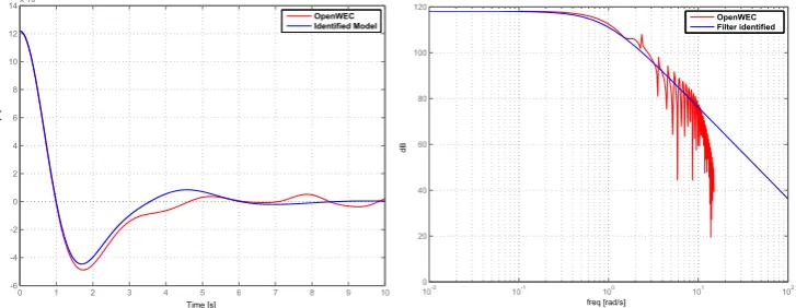
Figure 1.Comparative of the identified transfer functions: (a) Impulse response for radiation force

Kr(s). (b) Bode diagram for excitation forceFe(s).

To identify the WAP system, the openWEC software has been used [28]. Among other data, it 100

returns: the added water mass (m_∞ =167700 kg), the impulse response of the radiation force as a 101

function of the oscillation velocity and the frequency response of the excitation force. From these data, 102

the transfer function (9) is identified for the impulse response of the radiation force using the Prony 103

approximation [30]. On the other hand, the low-pass filter that defines the dynamics of the excitation 104

force caused by the incoming wave is tuned to the transfer function (10). The Figure1compares 105

the two transfer functions identified with the data delivered by the openWEC software. Finally, the 106

hydrostatic restoring coefficientkres=809325[N/m]is obtained using the Equation (5).

107

Kr(s) = Fr(s)

W(s) = aK8s

8_+a

K7s

7_+a

K6s

6_+a

K5s

5_+a

K4s

4_+a

K3s

3_+a

K2s

2_+a

K1s+aK0

s8_+b

K7s7+bK6s6+bK5s5+bK4s4+bK3s3+bK2s2+bK1s+bK0

N m/s

(9)

where the coefficientsaKandbKare listed in the Table1.

108

Fe(s)

η(s) =

6.5×105

(s+0.9)2

N m

(10)

Then, regrouping terms according to Equation (1), the transfer function (11) that relates external forces with the position of the buoy (z) is obtained.

GWEC(s) = Z(s)

Fext(s)

= a8s

8_+a

7s7+a6s6+a5s5+a4s4+a3s3+a2s2+a1s+a0 s10_+b

9s9+b8s8+b7s7+b6s6+b5s5+b4s4+b3s3+b2s2+b1s+b0 hm

N i

(11) where the coefficientsanandbnare listed in the Table1.

109

Table 1.Model coefficients identified for the WEC system.

Coefficient Value Coefficient Value Coefficient Value Coefficient Value

— — b9 88.49 — — — —

a8 2.443e-06 b8 1.462e05 aK8 1.218e03 — —

a7 2.162e-04 b7 6.681e06 aK7 2.297e05 bK7 88.492

a6 3.570e-01 b6 4.476e09 aK6 1.889e08 bK6 1.462e05

a5 16.32 b5 1.341e10 aK5 2.595e10 bK5 6.68e06

a4 1.093e04 b4 6.359e10 aK4 6.268e12 bK4 4.476e09

a3 3.268e04 b3 8.594e10 aK3 5.617e14 bK3 1.338e10

a2 1.304e05 b2 1.824e11 aK2 1.684e15 bK2 5.337e10

a1 1.353e05 b1 1.129e11 aK1 4.684e15 bK1 5.537e10

a0 1.599e05 b0 1.294e11 aK0 1.407e15 bK0 6.545e10

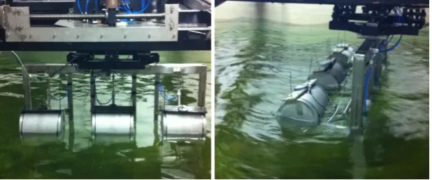
In order to validate the identification methodology proposed in this paper, the identification 110

process for the prototype of Figure3is carried out. Then, the response of the identified prototype 111

model is compared with the real response registered in [27]. For this purpose, to the identified model 112

the temporal series of forces recorded (see Figure2) are applied. 113

Figure 3.WEC prototype of the W2POWER platform, [27].

2.3. Treatment of the mathematical model for the design of MPCs 114

In order to ensure safe behaviour and reduce mechanical fatigue in PWAs systems, a model that 115

allows to be imposed constraints on the oscillation speed and position of the buoy is necessary. For this 116

reason, a brief study of the identified model (11) is needed. By representing in the state space, it can 117

be verified that the system obtained is not completely controllable, and therefore, it is not a minimal 118

realization [32]. Furthermore, it is not enough to reduce the model (11) to its minimum order, since, 119

except for the system output (z), the other state variables lack physical sense and this does not allow to 120

impose directly speed constraints (w). As a solution, we study the transfer function (9) that defines 121

the dynamics of the radiation force. Representing (9) in the state space, it can be seen how the model 122

obtained is not of minimum order. Therefore, the system is minimized by obtaining (12). Note that the 123

state variables of this model (xr) will not be controlled, so it is not necessary that they have physical

124

sense. 125

˙

xr(t) =Arxr(t) +Brw(t)

FrKr(t) =Crxr(t) +Drw(t)

(12)

where the matrixAr,Br,CryDrare given by (13).

Ar =     

−3.0044 −1.4736 −0.3820 −0.2258 8.1656 0.0180 0.0041 0.0025 0.0015 4.0015 0.0004 0.0002

−0.0000 −0.0000 2.0000 −0.0000 

   

, Br=

     121.3816 −1.3375 −0.1201 0.0005     

Cr =103

1.0083 0.3683 0.2624 0.0377, Dr =1218.70

(13)

A realistic model must consider the dynamics of the power take-off system. Given the similarity 127

between the Wavestar system and the WEC studied in this work, the PTO model proposed in [22] 128

is used, where the dynamics of the PTO is modeled according to (8). By representing this model in 129

the state space, with the parameters indicated in [22], we obtain the matrix (14), where observable 130

canonical form has been chosen. Thus, one of the state variables corresponds to the output of the PTO, 131

so it is possible for MPC controllers to impose restrictions on the output of the actuator. 132

Apto=

−8.7965 1.0000

−157.9137 0 !

, Bpto= 0

157.9137 !

, Cpto =

1 0, Dpto =0 (14)

After that, in this paper we propose (15) as one of the design models. On this model an MPC 133

controller can impose restrictions on the following state variables: force applied by the PTO (xpto1),

134

speed (w) and buoy position (z). This model is similar to the one proposed in [8,12], but also considering 135

the dynamics of the PTO system. 136           ˙ z ˙ w ˙ xr ˙ xpto          

| {z } ˙ x =             

0 1 0 0

−kres

mT

− 1

mTDr

− 1

mTCr

1 mTCpto

0 Br Ar 0

0 0 0 Apto

            

| {z }

A_WEC           z w xr xpto          

| {z }

x +           0 0 0 Bpto          

| {z }

B_WECu

Fu+

           0 1 mT 0 0           

| {z }

B_WECFe Fe    z w   

| {z }

y

= 

 

1 0 0 0

0 1 0 0



 

| {z }

CWEC           z w xr xpto          

| {z }

x

(15)

wheremT = m+m∞, the matricesI(unit matrix) and 0 have the required size according to their

137

location and the parameters not yet presented are listed in the Table2. 138

Table 2.Parameters of the models (15) and (16) for the WEC system.

Symbol Description Value

kres Hydrostatic restoring coefficient 809325N/m

Baprox Stationary approximation to system damping 21497Ns/m

m Mass of water displaced by the buoy at rest 241601.9kg

2.3.1. Simplified model for the design 139

For the design of some MPCs we use a simplified model (16). It differs from the previous model 140

(15) in that it does not consider the dynamics of the radiation force or the PTO system. Modeling 141

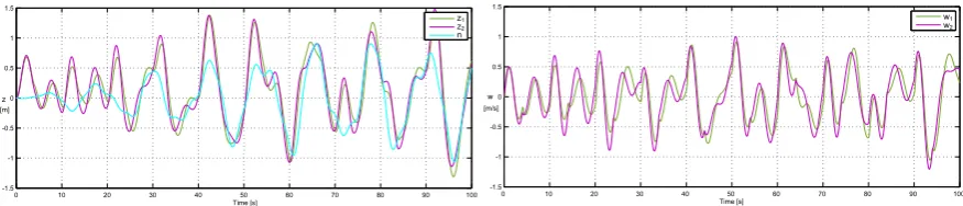
used in [9–11,13,14]. The Figure4shows a comparison of the outputs of the simplified model and the 142 complete model. 143     ˙ z ˙ w    

| {z } ˙ x =      0 1

−kres

mT

−Baprox

mT     

| {z }

AWECr     z w    

| {z }

x +      0 1 mT     

| {z }

BWECr

(Fu+Fe)

   z w   

| {z }

y =    1 0 0 1   

| {z }

CWECr     z w    

| {z }

x

(16)

wheremT =m+m∞and the parameters are listed in the Table2.

144

3. Model Predictive Control for Point Absorber Wave 145

This section details the design of the commonly used MPC controllers for PWAs. Moreover, in 146

this work two MPCs are proposed based on the addition of an embedded integrator. In order to make 147

a complete design, all the MPCs designed take into account constraints and the possibility of relaxing 148

them in the case of non-feasibility in the cost function. In particular, these constraints are applied to the 149

control force of the PTO system, the position of the buoy and its oscillation speed. However, in case of 150

non-feasibility, only soft-constrains are applied to the position and speed of the system. Because the 151

PTO is an actuator whose physical limit cannot be exceeded. Finally, for each controller a sampling 152

period ofTmis set, which is used to discretize the mathematical model employing the transformedz 153

zero-order-hold. 154

3.1. MPC1 155

The cost function that minimizes this controller directly considers the maximization of extracted 156

power. As a design model it uses (16), for which the state vector estimated for a prediction horizonM 157

and a control horizonNis defined according to Equation (17), [18,19]. 158 X=         A A2 A3 .. . AM        

| {z }

Jx(Mn×n) xk+

       

B 0 0 . . . 0

AB B 0 . . . 0

A2_{B AB B . . . 0}

..

. ... ... . .. ...

AM−1_{B A}M−2_{B A}M−3_{B . . . A}M−N_B

       

| {z }

Ju(Mn×N)

(Fpto+Fe) (17)

whereXrepresents the estimated state vector for a prediction horizonM,xkrepresents the state vector

159

at the current instant, the matricesAandBare obtained from the model (16) discretized,nis the order 160

of the model and,FptoandFeare vectors that contain the force applied by the PTO and the excitation

161

force for whole control horizonN, respectively. 162

In a more reduced form, the above equation can be expressed as: 163

0 10 20 30 40 50 60 70 80 90 100 -1

-0.5 0 0.5 1 1.5 2 2.5 3 3.5 4x 10

5

-1.5 -1 -0.5 0 0.5 1 1.5

z1

z2

n

F_u F_pto

0 10 20 30 40 50 60 70 80 90 100

Time [s] z

[m]

0 10 20 30 40 50 60 70 80 90 100

-1 -0.5 0 0.5 1 1.5 2 2.5 3 3.5 4x 10

5

-1.5 -1 -0.5 0 0.5 1 1.5

F_u F_pto

0 10 20 30 40 50 60 70 80 90 100

w1

w2

Time [s]

w

[m/s]

Figure 4.Comparison of models: complete (z1,w1) vs simplified (z2,w2). The height of the wave isn.

On the other side, the mechanical power generated is given by (19) [10,12,24]. Expressing the 164

power generated for the entire prediction horizon is obtained (20). 165

Pgen(t) =−Fpto(t)w(t) (19)

Pgen =−WTFpto (20)

whereWandFptoare vectors with lengthM, which represent the speed and control force for the entire

166

prediction horizon, respectively. 167

By replacing (18) in (20),

Pgen =−(SwX)TFpto

Pgen =−(Sw(Jxxk+JuFpto+JuFe))TFpto

(21)

whereSwis a selector matrix for speedw(sizeM×Mn).

168

Developing (21) and grouping in terms of least squares is obtained the cost function: 169

J(Fpto) = 1

2Fpto

T_(J

uTSwT+R)

| {z }

H

Fpto+1

2(Fe

T_J

uTSwT+xkTJxTSwT)

| {z }

b

Fpto ₍₂₂₎

where the matrixRweights the control effort. 170

In addition, constraints are imposed to: force demanded to the PTO, position and speed of the 171

buoy (24). Therefore, the cost function (22) with constraints is defined as: 172

J(Fpto) =1

2Fpto

T_HF

pto+1

2bFpto AgFpto≤Bg

(23)

whereAg= [A1 A2 A3]TyBg= [B1 B2 B3]T, see Equation (24). 173

" I

−I #

| {z }

A1

Fpto≤

"

FPTOmax

−FPTOmin

#

| {z }

B₁

, "

SzJu

−SzJu

#

| {z }

A2

Fpto ≤

"

Znmax−Sz(Jxxk+JuFe)

−Zn_min+Sz(Jxxk+JuFe)

#

| {z }

B2

" SwJu

−SwJu

#

| {z }

A3

Fpto≤

"

Wnmax−Sw(Jxxk+JuFe)

−Wn_min+Sw(Jxxk+JuFe)

#

| {z }

B3

(24)

whereSzis a selector matrix for position (sizeM×Mn), the vectorsFPTOmax andFPTOmin(sizeN×1)

174

define the nominal limits of the force applied by the PTO, the vectorsWnmax,Wnmin,Znmax andZnmin

175

(size M×1) define the nominal limits of the buoy position and oscillation speed, respectively. In 176

In the case of non-feasibility are applied soft constraints to the position and speed of the system. 178

So, the cost function (22) would be defined as: 179

J(Fpto,εz,εw) = 1

2Fpto

T_HF

pto+bFpto+εzTWεzεz+εw

T_W

εwεw (25)

whereεzandεwrepresent the relaxation applied to position and speed along the prediction horizonM

180

and the matricesWvarepsilonzandWvarepsilonw (sizeM×M) weight these slacks.

181

182

By regrouping terms and adding soft restrictions (27), the cost function (25) can be expressed as: 183

J(β) =1

2β

T



 

H 0 0

0 Wεz 0

0 0 Wεw



 β+

h

b 0 0iβ

Agβ≤Bg

(26)

where β = [Fpto εz εw]T, with size (N+2M)×1, Ag = [A1 A2 A3 A4 A5]T and Bg =

184

[B1 B2 B3 B4 B5]T, see Equation (27). Matrices 0 have the required size according to their 185

location. 186

"

SzJu −I 0

−SzJu −I 0

#

| {z }

A2

β≤

"

Znmax−Sz(Jxxk+JuFe)

−Zn_min+Sz(Jxxk+JuFe)

#

| {z }

B2

, "

SwJu 0 I

−SwJu 0 I

#

| {z }

A3

β≤

"

Wnmax−Sw(Jxxk+JuFe)

−Wn_min+Sw(Jxxk+JuFe)

#

| {z }

B3

"

I 0 0

−I 0 0 #

| {z }

A₁

β≤

"

FPTOmax

−FPTOmin

#

| {z }

B1

, "

0 I 0

0 −I 0 #

| {z }

A₄

β≤

"

κz

0 #

| {z }

B4

, "

0 0 I

0 0 −I #

| {z }

A5

β≤

"

κw

0 #

| {z }

B5

(27) whereκz andκw are vectors (size M×1) that represent the maximum slack allowed for position

187

and speed, respectively. The matricesI(unit matrix) and 0 have the required size according to their 188

location. 189

3.2. MPC2 190

This controller uses the simplified model (16). Its cost function is based on maximizing the 191

extracted power by tracking a setpoint for the system speed (wre f) along a prediction horizonM,

192

J= (w˜−wre f)TQ(w˜−wre f) +FptoTRFpto (28)

whereQandRare diagonal matrices of size(M×M)and(N×N)that weight the tracking error and 193

the control effort, respectively. 194

195

Substituting (18) in (28), the cost function for this controller can be written as (29). 196

J(Fpto) = (Jxxk+JuFpto+JuFe

| {z }

f

−wre f)TQ(Jxxk+JuFpto+JuFe

| {z }

f

−wre f) +FptoTRFpto (29)

By developing the cost function (29) and grouping terms the following expression is obtained: 197

J(Fpto) =FptoT(JuTδJu+R)

| {z }

H

Fpto+2(f−wre f)TQJu

| {z }

b

Fpto+ (f−wre f)TQ(f−wre f)

| {z }

l

Note that the terml can be ignored when the cost function is minimized, because it does not depend on the variable to be optimized (Fpto), remaining:

J(Fpto) = 1

2Fpto

T_(JT

uδJu+R)

| {z }

H

Fpto+ (Jxxk+JuFpto+JuFe−wre f)TQJu

| {z }

b

Fpto (31)

The constraints imposed on this cost function can be expressed in the same way as in theMPC1 198

controller. Using (23) for hard constraints and (26) for soft constraints. On the other hand, the reference 199

trajectory or setpoint for the speed is defined by the approach proposed in [29],wre f =Fe/2Baprox.

200

3.3. MPC3 201

This is a contribution made in this work. This controller uses the simplified model (16) to which an 202

embedded integrator has been added according to the theory of predictive controllers in the state space 203

[18,19]. Its cost function is based on the maximization of the extracted power through the tracking 204

of a setpoint for the system speed. To add the integrator it is necessary to multiply the model (16) 205

discretized by the operator4=1−z−1_{. Regrouping terms, an extended state vector is defined as:} 206

"

4x(t+1) y(t+1)

#

| {z }

xe(t+1)

= "

A 0

CA I #

| {z }

Ae

"

4x(t) y(t)

#

| {z }

xe(t)

+ "

B CB

#

| {z }

Be

4Fpto(t) +4Fe(t)

y(t) =h0 Ii | {z }

Ce

"

4x(t) y(t)

#

| {z }

xe(t)

(32)

where the output vectory(t)is formed by the position and speed of the WEC system,4x(t)represents 207

the state vector increment, the matrices A, B and Care from the model (16) discretized and the 208

matrices 0 have the required size according to their location. 209

210

Using the extended model (32), the prediction of the outputs (z,w) is defined for a prediction 211

horizonMand a control horizonNaccording: 212

Y= 

      

CA CA2 CA3 .. . CAM



      

| {z }

F(2M×ne)

Xe+



      

CB 0 0 . . . 0

CAB CB 0 . . . 0

CA2B CAB CB . . . 0

..

. ... ... . .. ...

CAM−1B CAM−2B CAM−3B . . . CAM−NB 

      

| {z }

G(2M×N)

(4Fpto+4Fe) (33)

wherene = n+jrepresents the order of the extended model and jits number of outputs. In the

213

matricesA BandCthe sub-indexehas been omitted to get a clearer notation. 214

215

By adding the embedded integrator, this controller minimizes a cost function that gets the optimal 216

increase in control force (Fpto) for the full control horizonN,

217

J = (w˜−wre f)TQ(w˜−wre f) +4FptoTR4Fpto (34)

whereQandRare diagonal matrices of size(M×M)and(N×N)that weighs the tracking error and 218

the control effort, respectively. 219

Replacing the output prediction (33) in (34) and obviating the independent term of4Fpto:

J(4Fpto) =1

24Fpto

T_(GT

δG+R)

| {z }

H

4Fpto+ (Fxek+G4Fe−wre f)

T_QG

| {z }

b

4Fpto (35)

In addition, constraints are added to the demanded force on the PTO, position and speed of the 221

system (37). Therefore, the cost function (35) subject to the restrictions is defined as: 222

J(4Fpto) =1

24Fpto

T_H4F

pto+b4Fpto

Ag4Fpto ≤Bg

(36)

whereAg= [A1 A2 A3]TyBg= [B1 B2 B3]T, see Equation (37). 223

" T

−T #

| {z }

A1

4Fpto ≤

"

FPTOmax

−FPTOmin

#

| {z }

B1

, "

SzG

−SzG

#

| {z }

A2

4Fpto≤

"

Znmax−Sz(Fxek+G4Fe)

−Znmin+Sz(Fxek+G4Fe)

#

| {z }

B2

" SwG

−SwG

#

| {z }

A3

4Fpto≤

"

Wnmax−Sw(Fxek+G4Fe)

−Wnmin+Sw(Fxek+G4Fe)

#

| {z }

B3

(37)

whereSzandSware selectors matrices forzandw(sizeM×Mn),Tis a lower triangular matrix (size

224

M×N), the vectorsFPTOmax andFPTOmin(sizeN×1) define the nominal limits of the force applied by

225

the PTO, the vectorsWnmax,Wnmin,Znmax andZnmin(sizeM×1) define the nominal limits of the buoy

226

position and oscillation speed, respectively. In addition, the matricesI(unit matrix) and 0 have the 227

required size according to their location. 228

Furthermore, if the cost function is not feasible (36), sotf constraints are applied,

J(β) =1

2β

T



 

H 0 0

0 Wεz 0

0 0 Wεw



 β+

h

b 0 0iβ

Agβ≤Bg

(38)

whereAg= [A1 A2 A3 A4 A5]TyBg= [B1 B2 B3 B4 B5]T, see Equation (38). 229

"

T 0 0

−T 0 0 #

| {z }

A1

β≤

"

FPTOmax

−FPTO_min

#

| {z }

B1

"

SzG −I 0

−SzG −I 0

#

| {z }

A2

β≤

"

Znmax−Sz(Fxek+G4Fe)

−Znmin+Sz(Fxek+G4Fe)

#

| {z }

B2

, "

0 I 0

0 −I 0 #

| {z }

A4

β≤

"

κz

0 #

| {z }

B4

"

SwG 0 I

−SwG 0 I

#

| {z }

A3

β≤

"

Wnmax−Sw(Fxek+G4Fe)

−Wnmin+Sw(Fxek+G4Fe)

#

| {z }

B3

, "

0 0 I

0 0 −I #

| {z }

A5

β≤

"

κw

0 #

| {z }

B5

(39)

whereκz andκw are vectors (size M×1) that represent the maximum slack allowed forzandw,

230

3.4. MPC4 232

This controller is made using the model (15). The cost function that minimizes this controller is 233

directly focused on the maximization of extracted power. The matrix development needed to express 234

this controller as a least squares problem is analogous to that presented for controllerMPC1. Although, 235

when considering the dynamics of the PTO system the Equation (18) should be redefined as: 236

X=Jxxk+JuFpto+JfFe (40)

whereJxis a matrix already defined in the equation (17), while the matricesJuandJf are given by:

237

Ju=



      

Bu 0 0 . . . 0

ABu Bu 0 . . . 0

A2_B

u ABu Bu . . . 0

..

. ... ... . .. ...

AM−1_B

u AM−2Bu AM−3Bu . . . AM−NBu



      

Jf =



      

BFe 0 0 . . . 0

ABFe BFe 0 . . . 0

A2BFe ABFe BFe . . . 0

..

. ... ... . .. ...

AM−1BFe A

M−2_B

Fe A

M−3_B

Fe . . . A

M−N_B

Fe



      

(41)

whereA,BuandBFe are obtained by discretizingAWEC,BWECuandBWECFe of the model (15).

238

The cost function to be minimized by this controller can be expressed according to (42). Its 239

development is analogous to that carried out for the controllerMPC1. 240

J(Fpto) =1

2Fpto

T_(J

uTSwT+R)

| {z }

H

Fpto+1

2(Fe

T_J

fTSwT+xkTJxTSwT)

| {z }

b

Fpto ₍₄₂₎

In addition, the nominal constraints imposed on the system must be added, which are defined in 241

the same way as in the controllerMPC1, Equation (24). Although in this case, it must be considered 242

that the state vector prediction is given by Equation (40). Therefore, the cost function (42) subject to the 243

constraints is defined as: 244

J(Fpto) =1

2Fpto

T_HF

pto+1

2bFpto AgFpto≤Bg

(43)

whereAg= [A1 A2 A3]TyBg= [B1 B2 B3]T, see Equation (24). 245

Finally, in the case of non-feasibility in the function (48) soft constraints will be applied to the 246

system. These can be expressed in a similar way to the development shown for theMPC1Equation 247

(27). Although, in this case it must be considered that the prediction of the state vector is given by the 248

equation (40). Therefore, the cost function of this controller subject to soft constraints is given by: 249

J(β) =1

2β

T



 

H 0 0

0 Wεz 0

0 0 Wεw



 β+

h

b 0 0iβ

Agβ≤Bg

(44)

3.5. MPC5 251

This proposal is another contribution made in this work. This controller uses the model (15), 252

which an embedded integrator has been added according to the theory of predictive controllers in the 253

state space [18,19]. Its cost function to minimize is based on the maximization of the extracted power 254

through the tracking of a setpoint for the speed of the systemwre f. As in theMPC3, the state vector is 255

extended by adding an embedded integrator (32). Although when considering the dynamics of the 256

PTO system the prediction of the output vector for the full prediction horizonMis defined by: 257

Y=Gu4Fpto+Fxek+Gf4Fe

| {z }

f

(45)

whereFis a matrix already defined in Equation (33) and the matricesGuandGf are given by:

258

Gu=



      

CeBeu 0 0 . . . 0

CeAeBeu CeBeu 0 . . . 0

CeAe2Beu CeAeBeu CeBeu . . . 0

..

. ... ... . .. ...

CeAeM−1Beu CeAe

M−2_B

eu CeAe

M−3_B

eu . . . CeAe

M−N_B

eu



      

Gf =



      

CeBe_Fe 0 0 . . . 0

CeAeBe_Fe CeBe_Fe 0 . . . 0

CeAe2Be_Fe CeAeBe_Fe CeBe_Fe . . . 0

..

. ... ... . .. ...

CeAeM−1Be_Fe CeAeM−2Be_Fe CeAeM−3Be_Fe . . . CeAeM−NBe_Fe



      

(46)

whereBeu andBeFe are obtained by discretizing the matrices that define the inputs of (15) extended.

259

Analogous to controllerMPC3, the cost function to be minimized can be expressed according to: 260

J(4Fpto) = 1

24Fpto

T_(G

uTδGu+R)

| {z }

H

4Fpto+ (Fxek+Gf4Fe−wre f)

T_QG

u

| {z }

b

4Fpto (47)

In addition, it is necessary to add nominal constraints to the system (37), which are defined as 261

in the controllerMPC3. However, in this case it must be considered that the prediction of the system 262

outputs is given by (45). So, the cost function (47) subject to the constraint is defined as: 263

J(4Fpto) =1

24Fpto

T_H4F

pto+1

2b4Fpto Ag4Fpto≤Bg

(48)

whereAg= [A1 A2 A3]TyBg= [B1 B2 B3]Tsee Equation (37). 264

Furthermore, in case of non-feasibility in the function (47), soft constraints are used. The 265

soft-constrains are expressed analogous to the development made for controller MPC3 Equation 266

(39). Although, in this case the prediction of the system output is given by (45). Therefore, the cost 267

function of this controller subject to soft constraints is defined as: 268

J(β) =1

2β

T



 

H 0 0

0 Wεz 0

0 0 Wεw



 β+

h

b 0 0iβ

Agβ≤Bg

(49)

4. Study about performances and robustness 270

This section presents the results obtained from an in-depth study of the performance and 271

robustness of the five MPCs designs. This study assumes that the system state vector and excitation 272

force (Fe) for the whole prediction horizon (M) are known (note that this has the same effect in all

273

MPCs). For this reason, the simulations are performed in an irregular sea state formed by the fifteen 274

sinusoidal components listed in the Table3. In addition, a comparison of the robustness of the designed 275

MPCs is made, which focuses on the uncertainty added to the most significant identified parameters 276

of the WEC system (min f ty,Baproxandkres). Note that when modifying the physical parameters of

277

the WEC system the frequency response of the filter (10) is affected. Therefore, looking for a realistic 278

comparative, it would be necessary to identify a new filter (6) for each added uncertainty. Given the 279

high number of simulations required, applying different levels of uncertainty to each of the parameters, 280

this is not feasible. For this reason, in this work the Morison model (7) is used to defineFe, allowing to

281

modify more easily the excitation force caused by the wave in function of the added uncertainty. 282

Table 3.Sinusoidal components used for sea-state (values expressed in international units).

Component Amplitude Period Phase Component Amplitude Period Phase

s1 0.420 13.00 −π s9 0.200 9.00 0.00

s2 0.520 12.50 1.5π s10 0.180 8.50 π

s3 0.420 12.25 0.40 s11 0.200 7.50 0.10

s4 0.520 11.50 0.20 s12 0.150 6.50 −0.77

s5 0.450 11.25 0.11π s13 0.100 5.50 0.5π

s6 0.300 10.50 −1.50 s14 0.075 5.00 0.00

s7 0.500 10.00 −0.33 s15 0.020 3.70 0.12

s8 0.210 9.50 0.78 — — — —

Due to the WEC system of the W2POWER platform have not yet been built, so their operating 283

limits and physical limits are not available. Therefore, these limits have been chosen on the basis of 284

[12,15,16,22], whose WECs systems are similar to the system studied in this paper, see Table4. 285

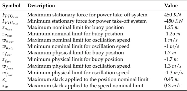
Table 4.Constraints for the WEC system.

Symbol Description Value

FPTOmax Maximum stationary force for power take-off system 450KN

FPTOmin Minimum stationary force for power take-off system -450KN

znmax Maximum nominal limit for buoy position 1.25m

znmin Minimum nominal limit for buoy position -1.25m

wnmax Maximum nominal limit for oscillation speed 1m/s

wnmin Minimum nominal limit for oscillation speed -1m/s

zfmax Maximum physical limit for buoy position 1.7m

zfmin Minimum physical limit for buoy position -1.7m

wfmax Maximum physical limit for oscillation speed 1.3m/s

wfmin Minimum physical limit for oscillation speed -1.3m/s κz Maximum slack applied to the position nominal limit 0.45m κw Maximum slack applied to the speed nominal limit 0.3m/s

All simulations have been carried out using MatLab/Simulink. In particular, they use the 286

Runge-Kutta integration method of order four (RK4) with an integration step of 1 ms and the function 287

quadprogof MatLab [33] to solve the cost functions with constraints. Note that although the quadprog 288

function providesFufor the entire control horizonN, only the setpoint obtained for the current instant

289

the tuning of all controllers, looking for the maximum possible veracity in their comparison. As a 291

result of this tuning, the parameters of the controllers are listed in the Table5. 292

Table 5.Design parameters set for each MPC controller (N=M).

Controller Tm[s] M R Q Wεz Wεw

MPC1 0.05 30 1.1×10−7 — 1.0×1010 1.0×107

MPC2 0.04 30 1.0×10−7 2.15×104 1.0×107 2.0×109

MPC3 0.04 30 5.0×10−5 1.475×104 5.0×1010 1.0×105

MPC4 0.05 30 4.5×10−7 — 1.0×108 1.0×104

MPC5 0.02 30 5.0×10−5 1.75×104 1.0×107 1.0×109

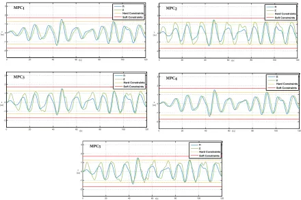
Figures5and6show a comparison between the heights and oscillations speeds obtained by 293

applying the five MPCs designs to the mathematical model (15). As can be seen, all controllers achieve 294

to keep the WEC system within its physical operating limits, even though the wave scenario chosen is 295

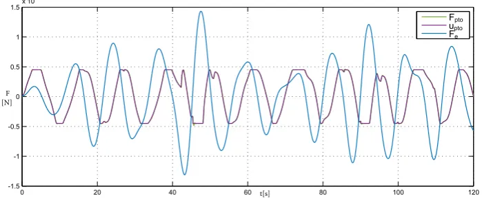
not favourable to the controllers. Because, as shown in Figure7, the wave force becomes more than 296

twice the stationary force that the PTO system can apply (recorded in the Table4). 297

0 20 40 60 80 100 120

-2 -1 0 1 2 3 -5 -4 -3 -2 -1 0 1 2 3 4 5 -1.5 -1 -0.5 0 0.5 1

1.5 Channel 1

Channel 1

n z

Soft Constraints

Time offset: 0

MPC1

Hard Constraints

z

[m]

t[s] 0 20 40 60 80 100 120

-2 -1 0 1 2 3 -5 -4 -3 -2 -1 0 1 2 3 4 5 -1.5 -1 -0.5 0 0.5 1

1.5 Channel 1

Channel 1

Time offset: 0

MPC2 n

z

Soft Constraints Hard Constraints

z [m]

t[s]

0 20 40 60 80 100 120

-2 -1 0 1 2 3 -5 -4 -3 -2 -1 0 1 2 3 4 5 -1.5 -1 -0.5 0 0.5 1

1.5 Channel 1

Channel 1

Time offset: 0 z [m] n z Soft Constraints Hard Constraints MPC3

t[s] 0 20 40 60 80 100 120

-2 -1 0 1 2 3 -5 -4 -3 -2 -1 0 1 2 3 4 5 -1.5 -1 -0.5 0 0.5 1

1.5 Channel 1

Channel 1

Time offset: 0 z [m]

t[s]

MPC4 n

z

Soft Constraints Hard Constraints

0 20 40 60 80 100 120

-2 -1 0 1 2 3 -5 -4 -3 -2 -1 0 1 2 3 4 5 -1.5 -1 -0.5 0 0.5 1

1.5 Channel 1

Channel 1

Time offset: 0

n z Soft Constraints Hard Constraints MPC5 z [m] t[s]

Figure 5.Comparison of the heights obtained in the WEC system when applying in simulation the five MPCs to the mathematical model (15).

On the other hand, the Figure8shows a comparative of the instantaneous mechanical powers 298

generated by applying the MPCs designed in this work. In this comparative, it can be seen how 299

applying theMPC2controller to the system gives the most irregular power. While the power generated 300

with theMPC3controller, designed from the same model and following the same optimization criteria, 301

is more clean. This is due to the fact that theMPC1controller is continuously applying soft constraints, 302

because it does not carry out a good control of the force that the PTO system exerts on the WEC along 303

integrator (controllerMPC3) considerably improves the behavior of the system with respect to that 305

obtained by applying the controllerMPC2. Because, theMPC3only exceeds the nominal limits of the 306

position and oscillation speed on one occasion. In addition, theMPC3controller generates a clearer 307

control signal than theMPC2(see Figure7) and, as a consequence, the underdamped response of the 308

PTO system decreases greatly. With this said, it can be concluded that the addition of the embedded 309

integrator to the design model improves the performance of the WEC device with respect to: quality 310

of the instantaneous power generated and reduction of mechanical fatigue (due to exceeding nominal 311

limits). 312

0 20 40 60 80 100 120

-1.5 -1 -0.5 0 0.5 1 1.5 2 -5 -4 -3 -2 -1 0 1 2 3 4 5 -1.5 -1 Channel 1

Time offset: 0

MPC1 w

Hard Constraints Soft Constraints

w [m/s]

t[s] -1.50 20 40 60 80 100 120

-1 -0.5 0 0.5 1 1.5 2 -1 -0.8 -0.6 -0.4 -0.2 0 0.2 0.4 0.6 0.8 1 -1 -0.8 -0.6 -0.4 Channel 1

Time offset: 0

MPC wref

6RIW&RQVWUDLQWV

Hard&RQVWUDLQWV

w

w

[m/s]

t[s]

0 20 40 60 80 100 120

-1.5 -1 -0.5 0 0.5 1 1.5 2 -1 -0.8 -0.6 -0.4 -0.2 0 0.2 0.4 0.6 0.8 1 -1 -0.8 -0.6 -0.4 -0.2 0 0.2 0.4 0.6 0.8 1 Channel 1 Channel 1

Time offset: 0

MPC3 wref

6RIW&RQVWUDLQWV

Hard&RQVWUDLQWV

w

w

[m/s]

t[s] -1.50 20 40 60 80 100 120

-1 -0.5 0 0.5 1 1.5 2 -1 -0.8 -0.6 -0.4 -0.2 0 0.2 0.4 0.6 0.8 1 -1 -0.8 -0.6 -0.4 -0.2 0 0.2 0.4 0.6 0.8 1 Channel 1 Channel 1 w Hard Constraints

Time offset: 0

MPC4

w [m/s]

t[s]

Soft Constraints

0 20 40 60 80 100 120

-1.5 -1 -0.5 0 0.5 1 1.5 2 -1 -0.8 -0.6 -0.4 -0.2 0 0.2 0.4 0.6 0.8 1 -1 -0.8 -0.6 -0.4 -0.2 0 0.2 0.4 0.6 0.8 1 Channel 1 Channel 1 wref 6RIW&RQVWUDLQWV

Time offset: 0

MPC5

w

[m/s]

t[s]

Hard&RQVWUDLQWV

w

Figure 6.Comparison of the oscillation speed obtained in the WEC system when applying in simulation the five MPCs to the mathematical model (15).

With respect to the generated power, controllers that use the full model (15) as the design model 313

get lower instantaneous power peaks than controllers that use the simplified model (16). This can be 314

verified comparing the MPCs that follow the same optimization criteria but are based on different 315

design models; the controllerMPC1withMPC4and the controllerMPC3withMPC5. Specifically, the 316

MPC5controller gets the best results, an average power of 97.04kWwhich rarely has punctual peaks. 317

Table 6. Results obtained in the application of the five MPCs to the WEC system. The powers are expressed inkW. Note thatONLPindicates Overshoot of Nominal Limits for Position andONLS

indicates Overshoot of Nominal Limits for Speed.

Controller Pgen¯ ON LH ON LS PgenMax PgenMin

MPC1 88.94 0.0054 0.0023 785.5 -491.7

MPC2 82.04 0.0259 0.0549 744.2 -369.4

MPC3 97.58 0.0137 0.0100 507.3 -379.0

MPC4 83.84 0.0156 0.0000 614.6 -237.3

17 of 22

0 20 40 60 80 100 120

-1.5 -1 -0.5 0 0.5 1 1.5x 10

6 -1 -0.8 -0.6 -0.4 -0.2 0 0.2 0.4 0.6 0.8 1 -1 -0.8 Channel 1

Time offset: 0

MPC1

F [N]

t[s]

Fpto

upto

Fe

0 20 40 60 80 100 120

-1 -0.5 0 0.5 1 x 106

-1 -0.8 -0.6 -0.4 -0.2 0 0.2 0.4 0.6 0.8 1 -1 -0.8 Channel 1

Time offset: 0

MPC

F [N]

t[s]

Fpto

upto

Fe

0 20 40 60 80 100 120

-1 -0.5 0 0.5 1 x 106

-1 -0.8 -0.6 -0.4 -0.2 0 0.2 0.4 0.6 0.8 1 -1 -0.8 -0.6 -0.4 -0.2 0 0.2 0.4 0.6 0.8 1 Channel 1 Channel 1

Time offset: 0

MPC3 F [N] t[s] Fpto upto Fe

0 20 40 60 80 100 120

-1 -0.5 0 0.5 1 x 106

-1 -0.8 -0.6 -0.4 -0.2 0 0.2 0.4 0.6 0.8 1 -1 -0.8 -0.6 -0.4 -0.2 0 0.2 0.4 0.6 0.8 1 Channel 1 Channel 1 Fpto upto Fe

Time offset: 0

F [N]

MPC4

t[s]

0 20 40 60 80 100 120

-1 -0.5 0 0.5 1 x 106

-1 -0.8 -0.6 -0.4 -0.2 0 0.2 0.4 0.6 0.8 1 -1 -0.8 -0.6 -0.4 -0.2 0 0.2 0.4 0.6 0.8 1 Channel 1 Channel 1

Time offset: 0

MPC5

F [N]

t[s]

Fpto

upto

Fe

Figure 7. Comparisons between: wave force, force setpoint demanded to the PTO and real force produced by the PTO, by applying in simulation the five MPCs to the model (15).

20 40 60 80 100 120 -500 0 500 1000 P (kW) MPC₁

20 40 60 80 100 120 -500 0 500 1000 P (kW) MPC₂

20 40 60 80 100 120 -500 0 500 1000 P (kW) MPC₃

20 40 60 80 100 120 -500 0 500 1000 P (kW) MPC₄

20 40 60 80 100 120 -500 0 500 1000 P (kW) MPC₅

Figure 8.Instantaneous mechanical powers generated by applying in simulation the five MPCs to the mathematical model (15).

Preprints (www.preprints.org) | NOT PEER-REVIEWED | Posted: 28 September 2018 doi:10.20944/preprints201809.0556.v1

To support all that has been said previously, the Table6records the most significant quality 318

indicators of the control performed by each MPC. First, this table shows the average mechanical 319

powers generated by the WEC system when applying each controller. In this aspect, the MPC3 320

controller achieves to generate more power, followed very closely by theMPC5and with a bit more 321

distance by theMPC1controller. On the other side, the indicatorsONLPandONLSquantify the area 322

of overshoot of the nominal limits of the position and oscillation speed, respectively. The controllers 323

MPC1 and MPC4 are the ones that apply the least slack to the nominal limits, followed by the 324

controllerMPC5. Therefore, with respect to the two optimization criteria compared in this paper, it 325

can be concluded that the controllers that directly maximize the extracted power (MPC1andMPC4) 326

get less overshoot of the nominal limits. While the MPCs that use an optimization criterion based 327

on the minimization of the error between the oscillation speedwand a setpointwre f for the whole

328

prediction horizon (M) obtain a higher average power extraction. Finally, the last two columns of the 329

Table6show the maximum and minimum power peaks obtained when applying each controller. In 330

this aspect, theMPC1is the most unfavorable while theMPC5reports the best performance. Note that 331

these power peaks will cause an oversizing of: electrical machines, power electronics, accumulators.. 332

4.1. Robustness comparative 333

Another contribution of this work, and searching the greatest realism in the comparative of the 334

designed controllers, uncertainty is added in the complete system model (15) to the most significant 335

identified parameters (50). Added mass and dynamic of the radiation force, parameters that have been 336

obtained through the openWEC software. On the other hand, the hydrostatic restoring coefficientKres,

337

a nonlinear parameter that has been linearized during the modeling of the WEC system. 338

Fres(t) =−kres(1+4kres)z(t)

FrKr(s)

W(s) = (1+4B)Kr(s)

Frm∞(t) =m∞(1+4m∞)w(t)˙

(50)

where4represents the added uncertainty in each parameters. 339

340

In addition, as mentioned above, by defining the excitation force with Morison’s linear model 341

facilitates the robustness analysis. Therefore, when modifying the physical parameters of the system, 342

the external force that the wave causes on the system also varies. So, Equation (7) is redefined for this 343

analysis as: 344

Fe(t) =m∞(1+4m_∞)η¨(t) +B(1+4B)η˙(t) +kres(1+4kres)η(t) (51)

Note that for the same wave height, the excitation force can increase or decrease according to the 345

uncertainty added in each parameter. Therefore, there will be situations where, for the sea state defined 346

in the Table3, the controller cannot keep the system within its physical limits. Since, the actuation 347

force of the PTO system will be much lower than the excitation force. In this paper, this non-feasibility 348

situation will be considered as the robustness limit that the controller can support. This limit is defined 349

for the uncertainty added in each of the parameters (50). This non-feasibility situation with soft 350

constraints does not mean that the closed-loop system becomes unstable, but that the controller cannot 351

keep the WEC system within the physical limits defined in the Table4. In addition, in order to obtain a 352

more complete analysis of how this uncertainty affects the closed-loop system, the average powers 353

generated for each value of added uncertainty to each parameter are recorded. A large number of 354

simulations have been carried out for this purpose, all of them using an integration step of 1 ms and 355

-100 0 100 200 300 400 500 600 700 800 900 20

30 40 50 60 70 80 90 100 110

MPC₁ MPC₂ MPC₃ MPC₄ MPC

5

Variation Generated Power - Uncertainty Added Mass

Power

[kW]

Uncertainty [%] -100 0 100 200 300 400 500 600 700 800 900

20 30 40 50 60 70 80 90 100

110 Variation Generated Power - Uncertainty Damping

Power

[kW]

Uncertainty [%]

MPC₁ MPC₂ MPC

3

MPC

4

MPC

5

-100 -80 -60 0 20 40

-20 0 20 40 60 80 100 120

-40 -20

MPC₁ MPC

2

MPC₃ MPC

4

MPC

5

Power

[kW]

Uncertainty [%]

Variation Generated Power - Uncertainty Hydrostatic Stiffness

Figure 9.Variations of the average mechanical power generated in function of the added uncertainty to: added mass, damping coefficient and hydrostatic restoring coefficient.

Once the robustness study has been defined, the Figure9shows the results obtained in function 357

of the added uncertainties; feasible limits obtained for the five MPCs and the variation of their 358

mean power generated. With respect to the added uncertainty inmin f ty, the controllerMPC2is the 359

least robust. Meanwhile, theMPC1controller offers the best features in a power-robustness ratio. 360

However, it should be noted that when considering more reasonable added uncertainty values (interval 361

[−50, 50]%), theMPC5extracts significantly more power than the others. It should also be noted that 362

the controllers that directly maximize power in their cost function (MPC1andMPC4) have the most 363

predictable behavior with respect to the added uncertainty inm_∞. On the other hand, theMPC5offers 364

the best features with respect to the uncertainty added to the dynamics of the radiation force (up to 365

400%). In contrast, theMPC2gives very bad results in this respect. TheMPC1also gets good results, 366

because it achieves a practically constant power production despite variations of4_B. Finally, the 367

Figure9shows how the power generated by the different controllers varies according to the uncertainty 368

added to the hydrostatic restoring coefficient of the system. In this aspect, it can be appreciated how 369

the robustness of all the controllers is more limited. Because, if the value of the coefficientkresincreases,

370

the excitation force that the wave exerts on the system (51) increases proportionally. Therefore, the 371

margin of action of the PTO system decreases noticeably. Even so, the MPC5supports an added 372

uncertainty of 25%, again being the that provides the best robustness results. Note that, for such added 373

uncertainty, the excitation force becomes more than three times the force that the PTO system can apply 374

20 of 22

0 20 40 60 80 100 120

-1.5 -1 -0.5 0 0.5 1 1.5x 10

6 -1 -0.8 -0.6 -0.4 -0.2 0 0.2 0.4 0.6 0.8 1 -1 -0.8 -0.6 -0.4 -0.2

Channel 1

Time offset: 0

F [N]

t[s]

Fpto upto Fe

Figure 10. Comparisons between: wave force, force setpoint demanded to the PTO and real force produced by the PTO, by applying in simulation theMPC5. The model (15) has an added uncertainty to the hydrostatic restoring coefficient of 25%.

5. Conclusions 376

The interest in implementing MPCs in WECs systems is motivated by the need to increase the 377

productive/economic viability of these systems. For this reason, in this work five different predictive 378

controllers have been designed. All these controllers allow minimizing mechanical fatigue by limiting 379

the operating range of the WEC system by means of hard and soft constraints. The main contribution 380

of this work is the study of performance and robustness carried out for the five MPCs designed. This 381

study demonstrates how the addition of an embedded integrator to the design model improves the 382

performance of the WEC device referring to average power generated, quality of instantaneous power 383

generated, reduction of mechanical fatigue and robustness of the closed-loop system, in comparison 384

with the other MPCs. On the other hand, it has been proven that controllers using design models that 385

consider the dynamics of the PTO system and of the radiation force, obtain instantaneous power peaks 386

lower than those obtained by using simplified models. With respect to the two optimization criteria 387

compared in this paper, it can be concluded that controllers that directly maximize the extracted power 388

get less overshoot of the nominal limits. Whereas controllers that use an optimization criterion based 389

on the minimization of the error between the oscillation speed of the system and a setpoint obtain 390

a higher level of average power extraction. Moreover, in order to provide veracity to this study, in 391

this work an identified methodology for PAWs has been proposed and validated for a scale prototype 392

using experimental time series. 393

Author Contributions:Rafael Guardeño was responsible for designing the predictive controllers, studying them 394

and writing most of the paper. Agustín Consegliere performed the modeling of the WEC system, proposed the 395

identification methodology for PAW systems and performed its validation. Manuel J. Lopez reviewed all the work 396

done, proposed the comparative robustness and wrote part of the document. Furthermore, Manuel J. Lopez and 397

Agustín Consegliere proposed the control problems to solve using Model Predictive Control strategy. 398

Acknowledgments:Thanks to all ORPHEO project partners for giving us the opportunity and funds to research 399

in this promising field. 400

References 401

1. Pecher. A.; Kofoed, J. P.Handbook of Ocean Wave Energy, Sprinder Open, Boca Raton, USA, 2016, ISBN 402

978-3-319-39888-4. 403

2. The Ocean Energy Systems Technology Collaboration Programme, Available online: 404

www.ocean-energy-systems.org/index.php (accessed on 4 may 2017). 405

3. Pelagic Power, Available online: www.pelagicpower.no/about.html (accessed on 6 may 2017). 406

4. Falnes, J.Ocean Waves and Oscillating Systems, Cambridge University Press, New York, USA, 2002, ISBN 407

0-521-78211-2. 408

Preprints (www.preprints.org) | NOT PEER-REVIEWED | Posted: 28 September 2018 doi:10.20944/preprints201809.0556.v1

5. Drew, B.; Plummer, A. R.; Sahinkaya, M. N. A review of wave energy converter technology,J. Power Energy, 409

2009,223, 887-902, doi: 10.1243/09576509JPE782. 410

6. Valério, D.; Beirao, P.; Mendes, M. J. G. C.; Costa, J. S. da. Comparison of control strategies performance for a 411

Wave Energy Converter. In16th Mediterranean Conference on Control and Automation; 2008; ; pp. 773–778. 412

7. Li, G. Predictive control of a wave energy converter with wave prediction using differential flatness. In 413

Proceeding of the 54th IEEE Conference on Decision and Control; 2015; pp. 3230–3235.

414

8. Andersen, P.; Pedersen, T. S.; Nielsen, K. M.; Vidal, E. Model Predictive Control of a Wave Energy Converter. 415

InIEEE Conference on Control Applications; 2015; pp. 1540–1545.

416

9. Brekken, T. K. On Model Predictive Control for a point absorber Wave Energy Converter. InIEEE Trondheim

417

PowerTech; 2011; pp. 1–8.

418

10. Richter, M.; Magana, M. E.; Sawodny, O.; Brekken, T. K. a Nonlinear Model Predictive Control 419

of a Point Absorber Wave Energy Converter. IEEE Trans. Sustain. Energy, 2013, 4, 118-126, doi: 420

10.1109/TSTE.2012.2202929. 421

11. G. Li; M. R. Belmont, Model predictive control of sea wave energy converters - Part I: A convex approach for 422

the case of a single device,Renew. Energy,2014,69, 453-463, doi: 10.1016/j.renene.2014.03.070. 423

12. Cavaglieri, D.; Bewley, T. R.; Previsic, M. Model Predictive Control leveraging Ensemble Kalman forecasting 424

for optimal power take-off in wave energy conversion systems. InProceedings of the American Control

425

Conference; 2015; Vol. 2015–July, pp. 5224–5230.

426

13. Oetinger, D.; Magaña, M. E.; Member, S.; Sawodny, O. Decentralized Model Predictive Control for Wave 427

Energy Converter Arrays.Sustain. Energy, IEEE Trans.2014,5, 1099–1107, doi:10.1109/TSTE.2014.2330824. 428

14. Li, G.; Belmont, M. R. Model predictive control of a sea wave energy converter: A convex approach. InThe

429

International Federation of Automatic Control; IFAC, 2014; Vol. 19, pp. 11987–11992.

430

15. Soltani, M. N.; Sichani, M. T.; Mirzaei, M. Model Predictive Control of Buoy Type Wave Energy Converter. 431

InThe International Federation of Automatic Control; IFAC, 2014; Vol. 47, pp. 11159–11164.

432

16. Starrett, M.; So, R.; Brekken, T. K. A.; McCall, A. Increasing power capture from multibody wave energy 433

conversion systems using model predictive control. InTechnologies for Sustainability; 2015; pp. 20–26. 434

17. Lagoun, M. S.; Benalia, A.; Benbouzid, M. E. H. A predictive power control of Doubly fed induction generator 435

for wave energy converter in irregular waves. In1st International Conference on Green Energy; 2014; pp. 26–31. 436

18. Camacho, E.F; BordonsC.Model Predictive Control, Sprinder, Sevilla, Spain, ISBN 978-1-85233-694-3. 437

19. Wang, L.Model Predictive Control System Desing and Implementation Using MATLAB, Sprinder, Melbourne, 438

Australia, 2009, ISBN 978-1-84882-330-3. 439

20. Bozzi, S.; Miquel, A. M.; Antonini, A.; Passoni, G.; Archetti R. Modeling of a point absorber for energy 440

conversion in Italian seas,Energies2013,6, 3033–3051, doi:10.3390/en6063033. 441

21. Hong, Y.; Eriksson, M.; Boström, C.; Waters, R. Impact of generator stroke length on energy production for a 442

direct drivewave energy converter.Energies2016,9, 1–12, doi:10.3390/en9090730. 443

22. Hansen, R. H.; Kramer, M. M. Modelling and Control of the Wavestar Prototype. InProceedings of the 9th

444

European Wave and Tidal Energy Conference; 2011; pp. 1–10.

445

23. Kovaltchouk, T.; Multon, B.; BenAhmed, H.; Glumineau, A.; Aubry, J. Influence of control strategy on the 446

global efficiency of a Direct Wave Energy Converter with electric Power Take-Off. InEighth International

447

Conference and Exhibition on Ecological Vehicles and Renewable Energies; 2013; pp. 1–10.

448

24. Fusco, F.; Ringwood, J. V A study of the prediction requirements in real-time control of wave energy 449

converters.IEEE Trans. Sustain. Energy,2012,3, 176 - 184, doi: 10.1109/TSTE.2011.2170226. 450

25. Tedeschi, E.; Carraro, M.; Molinas, M.; Mattavelli, P. Effect of control strategies and power take-off 451

efficiency on the power capture from sea waves. IEEE Trans. Energy Convers.,2011,26, 1088-1098, doi: 452

10.1109/TEC.2011.2164798. 453

26. Cummins W., The Impulse Response Function and Ship Motions, Schiffstechnick, 1962,9, 101-109, doi: 454

39080027544292. 455

27. Brandtsegg I., Validation of a Combined Wind and Wave Power Installation, Master, Norwegian University 456

of Science and Technology, Norway, 2014. 457

28. Openore, Available online: https://openore.org/2016/04/28/openwec/ (accessed on 14 may 2017). 458

29. Falnes, J.Ocean Waves and Oscillating Systems, Cambridge University Press, New York, USA, 2002, ISBN 459

0-521-78211-2. 460

31. Morison, J.R.; O’Brien M.P.; Johnson, J.W.; Schaaf, S.A. The forces exerted by surface waves on piles,Society

462

of Petroleum Engineers1950,189, 149-154, doi:10.2118/950149-G.

463

32. Ogata K. Ingeniería de control moderna, PEARSON EDUCACIÓN S.A., Madrid, Spain, 2010, ISBN 464

9788483226605. 465

33. Mathworks, Available online: https://es.mathworks.com/help/optim/ug/quadprog.html (accessed on 17 466