Abstract
Over the last 20 years genomics research has gained a lot of interest. Every year millions of articles are published and stored in databases. Researchers around the world want to be able to search for information about e.g. genes, diseases and enzymes. As of this moment there are no search methods available that give researchers a viable and efficient way to search for information about genomics data.
This Report discusses how information can be found using a desktop pc and a widely available database system. It will describe how the documents are found as well as the precision and recall of a query.
With the help of several well know Information retrieval methods, such as Boolean retrieval, TF*IDF and stemming, the effects of these searching methods will be tested, and compared to each other.
Preface
This paper is written as a conclusion to my studies at the University of Twente.
The genomics TREC was used as a basis for my gradation assignment. The Medline data and the questions they provided were used as a benchmark for the developed system.
I would like to thank dr.ir. D. Hiemstra and dr. P.E. van der Vet for their help and supervision during this project.
Utrecht, 2005
Table of contents
ABSTRACT... 2
PREFACE ... 3
TABLE OF CONTENTS ... 4
1 INTRODUCTION ... 7
2 VARIOUS SEARCH METHODS... 10
2.1 RETRIEVAL METHODS... 10
2.1.1 BOOLEAN RETRIEVAL... 10
2.1.2 BOOLEAN RETRIEVAL WITH TF*IDF ... 11
2.2 RETRIEVAL UTILITIES... 12
2.2.1 CLUSTERING... 12
2.2.2 PARSING... 12
2.2.3 THESAURI... 13
2.2.4 MULTI-WORD TERMS... 13
2.2.5 MESH TERMS... 13
3 RESEARCH DIRECTIONS... 14
3.1 THE DATA... 14
3.2 THE TOPICS... 15
3.3 THE METHOD... 15
4 APPROACH... 17
4.1 THESAURUS... 17
4.2 REMOVAL OF STOP WORDS... 17
4.3 STEMMING... 17
4.4 RANKING... 18
4.4.1 RANKING TYPE 1... 18
4.4.2 RANKING TYPE 2... 18
4.5 MULTI-WORD EXPRESSIONS... 18
5 IMPLEMENTATION ... 19
5.1 THE BASIC SYSTEM... 19
5.1.4 RANKING... 21
5.2 THESAURUS... 21
5.2.1 SEARCHING WITH THE THESAURUS... 21
5.3 STEMMING... 22
5.3.1 SEARCHING WITH STEMMING... 22
5.4 RANKING... 22
5.4.1 RANKING TYPE 1... 22
5.4.2 RANKING TYPE 2... 23
5.5 MULTI-WORD TERMS... 25
5.6 MESH TERMS... 26
5.7 CROSS-SOURCE SEARCHING... 27
5.8 QUERY TERMS... 28
6 JUDGMENT CRITERIA ... 29
7 RESULTS ... 30
7.1 THE DATABASE... 31
7.2 THESAURUS... 31
7.3 STOP WORDS... 32
7.4 EVALUATION OF THE QUERY TERMS... 33
7.5 STEMMING... 35
7.6 RANKING... 36
7.7 RANKING TYPES... 37
7.8 MULTI-WORD-TERMS... 38
7.9 COMPARISON OF QUERY TYPES... 39
7.10 MESH TERMS... 40
7.11 CROSS-SOURCE SEARCHING... 41
8 EVALUATION OF THE RESULTS ... 42
8.1 WHY IS THE EFFECT OF THE THESAURUS SO LIMITED?... 42
8.2 WHY IS THERE LITTLE DIFFERENCE BETWEEN THE RANKING TYPES? ... 42
8.3 WHY IS THE EFFECT OF SEARCHING MESH TERMS SO LIMITED?... 43
8.4 WHY IS THE OVERALL RECALL ONLY 47%? ... 43
8.5 WHY IS THE EFFECT OF CROSS-SOURCE SEARCHING SO LIMITED? ... 44
9 COMPARISON WITH OTHERS... 45
9.1 GENERAL COMPARISON... 45
9.2 COMPARISON AGAINST THE BEST RUN... 45
10 CONCLUSIONS AND FUTURE IMPROVEMENTS... 47
12 APPENDICES... 50
APPENDIX I–PUBMED FIELDS... 50
APPENDIX II–THE TOPICS... 53
APPENDIX III– STOP WORDS... 60
APPENDIX IV– PUNCTUATION SIGNS... 62
APPENDIX V–RECALL VALUES... 63
APPENDIX VI–MAP VALUES... 65
APPENDIX VII-P10 VALUES... 67
APPENDIX VIII-P100 VALUES... 69
APPENDIX IX-QUERY TERMS... 71
APPENDIX X-UPDATED QUERY TERMS... 72
1
Introduction
The Text REtrieval Conference (TREC) supports research within the information retrieval community. TREC has several branches (tracks) of research going every year. One of these tracks is the “Genomics Track“.
The Genomics track was introduced in 2003 and will run for at least 5 years. The purpose of the track is to study information retrieval in the genomics data domain (this includes not just gene sequences, but also documentation such as research papers, lab reports, etc).
For my graduation assignment I joined the 2004 genomics track, more specifically the “Ad Hoc Retrieval Task”.
The structure of this task is a conventional searching task based on a 10-year subset of MEDLINE (about 4.5 million documents and 9 gigabytes in size) and 50 topics derived from information needs obtained via interviews of real biomedical researchers. [008]
Over the last twenty years genomics research has expanded greatly. Every year thousands or articles, papers and journals are published. Most of these articles, papers and journals are included in the MEDLINE database. Despite the fact that almost all information is available, in electronic form; most people still rely on MEDLINE when searching for information. Because MEDLINE is the number one source of information, when searching for genomics information, the ability to search the MEDLINE database is getting more and more important. The Genomics track tries to find new and more efficient ways to search the genomics information.
Before we go into the goal of this paper, a closer look will be taken at the other participants of TREC. An overview will be given of the problems and expectations other researchers are having.
When examining the papers the other participants of the Genomics TREC submitted then there are three problems when searching the TREC database.
• Linguistic problems: synonymy and Homonymy
Researchers all over the world are using different terms for the same genes, conditions and/or effects.
• Automated query generation.
The topics provided by TREC are writing in natural language. How can the system atomically generate the query needed to find relevant information out of the topic?
Because of the thousands of articles, papers and journals that are being published the amount of information that has to be searched is huge.
Most of the participants of the Genomics TREC agree that synonymy is the biggest problem when searching for information. They don’t however agree on the way to overcome the problem. The solutions to the problem can however be categorized into 2 distinct categories.
• Use of a thesaurus.
Some participants use a precompiled thesaurus to match the different synonyms with each other [018] and [019].
• Relevance feedback.
Some participants look at the make up of articles that get a high ranking and expand they search terms with words that are likely to be synonyms of terms they are looking for [012] and [017].
The second problem that people are facing is the automated query generation. TREC gives its member the option to turn in both manual and automatic runs. Manual runs are runs where participants select their own query terms based on their interpretation of the natural langue and the terms they think are important to find information. On automatic runs the system itself will determine which terms it will use to find relevant information. There are several ways of generating automatic queries; a few of them are listed below.
• Using term frequency
Words in the topics that don’t occur at a high frequency in the database are more likely to be of value then words that occur frequently in the database [012] and [017].
• Using controlled vocabularies
Words that occur in medical dictionaries have a higher likeliness of being relevant. Also words that do not occur in a regular dictionary (proper English) have a high likely hood of being relevant [018] and [020].
After evaluating the problems the other participants identified there are two problems we will be focusing on in this paper.
• A huge dataset:
For this assignment 9 Gb of raw text needs to be searched.
• No clear naming schema for gene-names
Synonyms are a big problem when looking for information.
corrects itself when more search terms are added (the chance that a document contains a homonym of the term you are actually looking for diminishes with every term added).
2
Various search methods
In this chapter I will discuss several popular ways to retrieve data from a dataset. This chapter is divided in 2 sections. The first section will discuss several Retrieval methods. The second section will discuss several retrieval utilities which can be used with any retrieval method to improve the results.
2.1 Retrieval methods
In this section two retrieval methods are discussed. There are many more ways to retrieve data. I chose to only include to most commonly used methods. The methods that aren’t listed would either take too much time to implement or wouldn’t run efficiently on a desktop system.
Generally retrieval methods can be divided into two classes:
• Exact-match searching. This method only retrieves documents that match all the terms the user is looking for. Examples of exact match searching are Boolean search and Boolean TF*IDF search.
• Partial-match searching. This method retrieves all documents that match at least one of the search terms. The documents are then ranked by the system to ensure that documents that match the search criteria “better” are given a higher rank. Examples of partial match searching are fuzzy set, vector space, and probabilistic retrieval.
Because the search terms for the fifty topics, which TREC provided, are handpicked by the user, all the terms, which are searched for, are of great importance. This means that documents that do not satisfy at least one of the terms have a big chance of being irrelevant. This means the system will need Exact-match searching. In the following section two exact-match search methods are discussed.
2.1.1 Boolean retrieval
2.1.2 Boolean retrieval with TF*IDF
This method is actually an extension of Boolean retrieval. It was designed in order create a way to rank documents on relevance. The method assigns every term in the database a weight that can be used to judge the importance of that term (terms that occur few times in the database get a high relevance, common terms get a low relevance).
The method works like this:
• A list of documents is retrieved using the “normal” Boolean search.
• For every document o For every Term
§ Calculate the TF*IDF ranking of the term in the retrieved document
o Add all the TF*IDF rankings. This number is the relevance judgment for the document
• Order all the documents on their relevance value.
TF stands for “Term frequency” and IDF stands for “Inverse document frequency”. The formulas to calculate both TF and IDF are given below.
TF(term) = the frequency of a term in a document.
IDF (term, document) = IDF (term, document) = 0
If no documents are retrieved
The weight of a term in a document can be computed now.
Weight (term, document) = TF(term, document) * IDF(term)
The TF*IDF ranking discussed in this section is the most basic form of TF*IDF rankings. The ranking can be modified to use document specific information (e.g. document length) to further increase the precision of the ranking.
2.2 Retrieval utilities
In this section several retrieval utilities are discussed that can be used to improve results of the retrieval methods discussed in the previous section.
2.2.1 Clustering
Clustering tries to group documents by content. This reduces the search space needed by a query to respond. The biggest problem with clustering is the computational complexity. In order to assign every document a cluster the system needs to compare every document with all the other documents. Over the years a lot of methods were created to automate the clustering process. A detailed review of clustering algorithms is given in [013].
2.2.2 Parsing
Using parsing on the documents before they are being searched can improve performance and precision of the system. There are 3 ways to change the documents before they are added into the system:
• Removal of punctuation and case folding.
o This step usually improves both precision and performance of the system because it lowers the amount of terms available in the system and it decreases the chance of a word getting indexed twice (e.g. Iron-Regulator and ironregulator will both be indexed as ironregulator).
• Removal of stop words.
o Stop words are words that are used often in sentences but they don’t say very much about the meaning of the sentence. Removing these words can greatly decrease the amount of data stored in the database. But special care has to be taken to make sure no search terms occur in the stop words list.
• Stemming of the words.
o Stemming is a technique for reducing words to their grammatical roots. There is much discussion about the use of stemming in databases. It improves performance of system but it doesn’t always improve precision.
o The popular stemming algorithms are: § Lovins stemmer [014].
2.2.3 Thesauri
The definition of a Thesaurus:
A Thesaurus is a type of dictionary where groups of words with the same meaning are grouped together. [015]
When searching through documents it is often useful for the user to also find synonyms of the words he is looking for e.g. (car and automobile). A thesaurus can help a database system to expand a query so it also includes synonyms, of the search terms the user is looking for.
2.2.4 Multi-word terms
Multi-word terms are search terms that consist of more then one word (e.g. Iron-regulated transporter 1). Using a standard Boolean search the system would search for the separate words of the term and take the intersection of the results of all the separate words. When adding support for multi-word terms, the system will not just take the intersection of the separate words, but will also look at the proximity of the words. If the separate words of the query are not next to each other then the term as a whole will not be counted as a hit.
2.2.5 Mesh terms
3
Research directions
Now that the methods of searching though text documents are clear, we will look at the data and the questions that have to be answered.
3.1 The data
The data that will be used is provided as a 9 Gb text file. Every line of the file corresponds with a field from the MEDLINE database. A detailed list of possible fields in the text file can be found in appendix I. Out of all the fields it was decided to only use the abstract, title and mesh terms of every document. The other fields don’t give information about the content; they focus primarily on the authors, copyrights and the date and/or place of publishing.
In order to test reliability of the fields that will be used in the tests 10.000 random documents were selected and checked for their title, abstract and mesh term contents. Of all the documents in the test collection over 99% of them have a title defined, 65% has an abstract defined and about 80% has mesh terms defined
3.2 The topics
TREC provided its participants with a list of 50 topics that need to be answered. For every topic 4 fields are specified.
• ID - This is the number of the topic.
• Title - This is the title of the topic
• Need - This field describes what the user is supposed to search for
• Context - This gives background information why the information is needed.
The list of topics can be found in appendix II.
After examination of the topics they can be divided into 3 groups.
• Type 1
o topics of the form: find information about A in B (topics: 1, 3, 4 , 6, 9, 10, 11, 13, 14, 15, 18, 20, 21, 23, 26, 27, 31, 32, 34, 38, 39, 40, 44, 46, 47, 48, 50)
• Type2
o Topics of the form: find a protocol, method or function that describes C (topics: 2, 5, 12, 16, 17, 22, 24, 25, 29, 30, 33, 35, 36, 37, 41, 42, 43, 45, 49)
• Type3
o Topics of the form: find correlation between D and E (topics: 7, 8, 19, 28)
Where
• A is a protein, gene, disease or process
• B is an organism or a process
• C is a protein, gene, disease or process
• D is a protein, gene, disease or process
• E is a protein, gene, disease or process
3.3 The method
After looking at the data and the topics I’ve decided to use Boolean searching for the database. This was done because of the need to search for just a few terms per topic and all terms should be present in the document in order for the document to be relevant. Other searching methods (like probabilistic or vector based searching) could also be used but the extra resources needed for those systems are simply not needed when searching terms of equal importance.
specified in section 3.2, then the chances of the document being relevant are very slim.
Once Boolean searching was set it was decided to use the PostgreSQL database system [009]. This system was chosen for several reasons.
• It is widely available for download on the internet.
• It has support to run on Microsoft Windows, the operating system that is running on the desktop pc used to create the system.
• Support for big tables (a table limit of 16 Terabyte).
• Proven stability and performance; postgreSQL has been around since 1987 and has proven itself during the years of its development.
• Excellent support to create stored procedures.
To optimize performance and precision the following utilities will be used:
• TF*IDF
• Parsing.
• Stemming.
• Removal of stop words.
• Removal of punctuation.
• Thesaurus
• Clustering
• Mesh terms
4
Approach
In order to test the effect of the various searching utilities several test runs were conducted. First a database was created that only used the removal of punctuation and clustering. The results we got from this database were used to test the effect of adding several Utilities. New utilities were added to the system every run. After every run the results of that run were compared to the best run up to that moment, if the results had improved the utility was used in all the following runs. If the results had decreased the utility was dropped.
At first only the title and abstract fields of the documents were searched. Once the optimal searching methods for those fields were decided, the effect of adding a search of the mesh terms was added. This was done to limit the amount of data the system had to search.
4.1 Thesaurus
The first addition to the system was a thesaurus. The thesaurus was manually filled with data. The data was retrieved from the “Entrez gene” database [006], and contains synonyms and abbreviations of terms used to search the database. Of the fifty topics provided by TREC only ten contain terms that can be expanded by looking at the “Entrez gene” database. Therefore the effect the thesaurus had on the results was limited to those ten topics.
4.2 Removal of stop words
The second addition to the system was the removal of stop words. The list of stop words I choose to use is the same list of stop words that’s used by the MEDLINE database. The list was created by selecting the words that occur most in the database. Because of the huge amount of hits these words would generate they are useless to use in a query. To be certain, no important words were dropped. The list of fifty topics was compared with the stop words and none of the topics included a search term that was included in the list of stop words. A list of the words that will be removed can be found in Appendix II.
4.3 Stemming
4.4 Ranking
Two types or ranking were used. In the following sections both will be discussed. During the first test the effect of using ranking of type 1 was tested.
4.4.1 Ranking type 1
This is a very basic ranking system; all terms that are found have the same importance. The system calculates how often the terms the user is looking for are used in both the title and the abstract and awards 3 point to a hit in the title and 2 points to a hit in the abstract.
4.4.2 Ranking type 2
During the third test a modified TF*IDF system was added. The system does not look at individual terms when creating the weight of a term, but looks at all synonyms of a word as if they are one word. The modified system works like this:
TF(term) = the frequency of a term in a document.
TF(term) total = sum of all TF(term) where the terms are synonyms
IDF (term, document) total = IDF (term, document) total = 0
if no document and synonyms are found.
The weight of a term and its synonyms in a document can be computed now. Weight(term, document) total = TF(term, document) total * IDF(term) total
It was decided to use the most basic form of TF*IDF ranking, this is because it minimizes the computational complexity but still gives a good comparison between the two ranking types. If eventually we want to optimize the results then different ways of expanding the TF*IDF system can be considered.
4.5 Multi-word expressions
5
Implementation
In this chapter an explanation will be given on how the utilities discussed in the previous chapter can be implemented. In the first section the basic system without any of the features will be discussed. The sections following 5.1 will discuss how the utilities discussed in the previous chapter will be implemented. For every utility added it is assumed that the utilities discussed in the sections before the one being discussed are all implemented.
5.1 The basic system
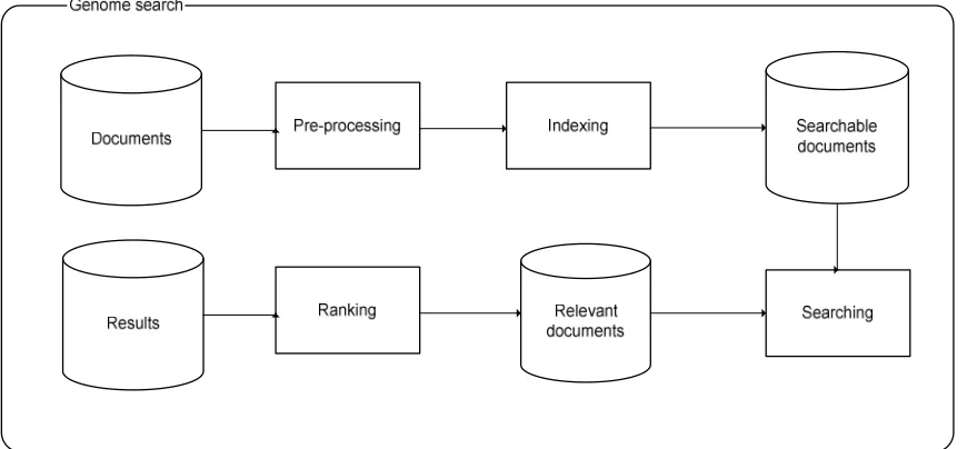
The system is depicted in figure 5.1. As can be seen the system contains four processes.
• Pre-processing
• Indexing
• Searching
• Ranking
The first two steps, pre-processing and indexing, are only preformed once, when the database is being initialized. After its initialization the database will be ready to be used. In this chapter all the steps needed to create the database and to get results from it will be discussed. All these steps have to be taken for both the title and the abstract of a document. In the next sections the four processes are explained.
5.1.1 Pre-processing
During this step all characters will be converted to lowercase and all punctuation signs and stopwords will be deleted. The removal of punctuation signs will follow the rules as they are set in Appendix IV.
5.1.2 Indexing
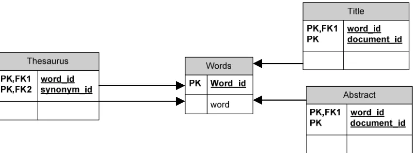
During this process all the documents are put into the database. Figure 5.2 shows the database schema of the database. The indexing process both indexes the abstract and the title fields of the dataset. Both fields are stored in a separate table. The indexing process will give every word it encounters, in the dataset, a unique id. Then for every document a list with the document id and the word id is stored in either the abstract or title table.
Figure 5.2 – Database schema of the database
5.1.3 Searching
During the searching process the system attempts to retrieve as many relevant documents as possible. It attempts to do this in the following way. At this point the system does not support multi-word terms, the words of multi-word terms are treated as separate terms.
• System receives a query with X terms
• For every X retrieve the word id(W) of X
• For every X retrieve the document ids from both the title and abstract tables of the documents that contain W.
At the end of this process the system will have a list of all documents containing all the terms.
5.1.4 Ranking
During the ranking process documents are listed in order of importance. The basic system does not have any sort of ranking, so during the ranking process the data will not be changed. This process was included in figure 5.1 because it will be needed in future improvements discussed in the following sections.
5.2 Thesaurus
In order to make use of a thesaurus the database schema (figure 5.2) has to be changed. The new database schema is given in figure 5.3. The thesaurus is manually generated after the system is about to finish the indexing process.
Figure 5.3 – Database schema including a thesaurus
As can be seen in figure 5.3 the thesaurus contains a list of word ids. It is basically linking words together if they are synonyms.
5.2.1 Searching with the thesaurus
During the searching process the system attempts to retrieve as many relevant documents as possible. It attempts to do this in the following way.
• System receives a query with X terms
• For every X retrieve the word id(W) of X
• For every W retrieve synonyms Y from the thesaurus
• For every X retrieve the document ids from both the title- and abstract tables of the documents that contain W or Y.
• Take the Intersection of all the documents retrieved for every X.
5.3 Stemming
Like the removal of stop words, stemming will be added in the pre-processing stage, but it will be put between the removal of punctuation and the removal of stop words. This is because stemming might result in more stop words appearing in the document. These stop words then have to be removed.
Stemming has no influence on the design of the database. The database remains as depicted in figure 5.3. Stemming does have a small impact on the searching process. Therefore the searching process will be modified.
5.3.1 Searching with stemming
During the searching process the system attempts to retrieve as many relevant documents as possible. It attempts to do this in the following way.
• System receives a query with X terms
• For every X calculate its stem(S)
• For every term X retrieve the word id(W) of S
• For every W retrieve synonyms Y from the thesaurus
• For every term X retrieve the document ids from both the title- and abstract tables of the documents that contain W or Y.
• Take the Intersection of all the documents retrieved for every X.
At the end of this process the system will have a list of all documents containing all the stemmed terms and/or their stemmed synonyms.
5.4 Ranking
In this section the implementations of both the ranking types discussed in section 6.4 are discussed.
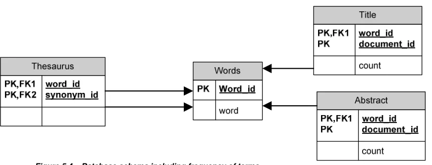
5.4.1 Ranking type 1
Figure 5.4 – Database schema including frequency of terms
Figure 5.4 shows that for every document and word the system now counts how many times a word occurs in either the title or the abstract.
The searching process remains unchanged but Instead of just returning a list of documents that match all the terms, the search process will now return a list of all documents that match the terms, but will also return the amount of times every term occurs in the title and/or abstract.
After the search returns its results the ranking process (section 5.1.4) starts. The ranking process will award 3 points to every hit of a term in the title and 2 points for every hit in the abstract. After the ranking process finishes ranking all documents, it will order the list of documents according to rank and present the results to the user.
5.4.2 Ranking type 2
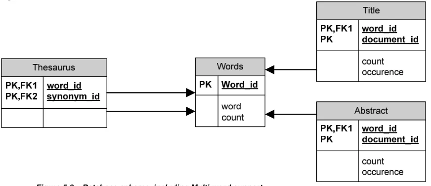
Ranking type 2 not only keeps track of the frequency in which a word occurs in a title and/or abstract. It also keeps track how frequently a word occurs in separate documents. In order to do so a frequency counter has to be added to the words table. The new database schema is shown in figure 5.5.
The searching process remains the same was with searching of type 1.
5.5 Multi-word terms
Instead of treating separate terms in multi-word terms as different terms, the system can attempt to guarantee that the words are in close proximity of each other before the terms are treated as a hit. The system will have to keep track of the location of a word in a title and/abstract. In order to do so the title and abstract tables will have to be expanded. The new database schema is shown in figure 5.6.
Figure 5.6 – Database schema including Multi-word support.
Figure 5.6 shows that both the title and abstract tables have a new column called “occurrence”. This column contains an array of positions at which a word occurs in the text.
Searching the database has to be changed a little, it now has to retrieve the list of relevant documents including the count and occurrence of each search term.
During the ranking process the actual checking of multi-word terms is done. The ranking engine will analyze each sub-term of the multi-word term and check if it is in close enough proximity of the other sub-terms. If it is not close enough, the system will remove the term from its results (effectively removing it from the occurrence list at the index where it used to be and decrease the term counter by one). After all terms have been checked, the ranking engine will start its usual ranking routine, ranking all the separate terms found.
5.6 mesh terms
All utilities in the previous sections only searched the title and the abstract of a document. In this section we will add the ability to search the mesh terms of the documents. In order to be able to do so a new table has to be added to the database design. The new database design is shown in figure 5.7.
Figure 5.7 – Database schema including mesh terms
5.7 Cross-source searching
With the database design as shown in Figure 5.7 there is a limitation, it is impossible to search for different search terms across different tables. In order to make it possible for the system, to search for all the different information about a document, the information has to be stored in one table and not in three separate tables. The modified database schema is shown in figure 5.8
Figure 5.8 – Database schema with combined information
5.8 Query terms
In section 3.2 the fifty topics provided by TREC were divided into 3 different types. In this chapter we will decide on the terms that will be used when searching for every topic.
There is not a strict set of rules that dictates which terms to use. Deciding on the terms is something that is done by human judgment, but the terms are roughly decided upon like this:
• Type 1
o Look for terms A and B
• Type 2
o Look for C
• Type 3
o Look for D and E
At this point there is no difference between how queries of type 1 and type 3 are handled. In section 7.4 a different set of query terms will be selected to improve performance, by then the difference between type 1 and type 3 will become apparent.
6
Judgment criteria
In order to test the effectiveness of our system, the results will be run though the TREC evaluation (“trec_eval”) program [010]. This program generates information about the performance of a system.
The program takes two input files:
• The results of a run
• A relevance file.
The relevance file is provided by TREC to all its participants. It contains a list of relevant documents for all the topics TREC provided. A complete explanation of how this list was created can be found in [011].
Once the TREC evaluation program has judged a run, the following numbers will be looked at:
• Percentage found (Recall): this number represents the amount of relevant documents found (a Recall of 0,45 means that 45% of all relevant documents were found). This number is not affected by the amount of irrelevant documents retrieved, nor is it affected by the ranking documents have. This number only gives information about the recall of a run.
• Precision at 10 (P10): this number represents the number of relevant documents found in the 10 highest ranked documents. This number only gives information about the precision of a run.
• Precision at 100 (P100): this number represents the number of relevant documents found in the 100 most highly ranked documents. This number only gives information about the precision of a run.
• Mean average precision (MAP): The average precision of a single query is the mean of the precision scores after each relevant document retrieved. This number provides information about both the recall and the precision of a run.
More information about various measurements can be found in [005].
The TREC evaluation program provides several other numbers to measure the precision of a query. These will not be used. P10, P100 and MAP give a good enough view of the precision to compare the different methods. If in the future slight adjustments to the ranking system have to be tested, it is advised to also look at different measures.
7
Results
In order to research the actual effectiveness of the methods discussed in the previous chapters several tests were conducted. For every consecutive run one feature was added or removed to see the effectiveness of that feature. Table 7.1 shows which features were turned on at each individual run. The columns in the table represent a feature discussed in the previous chapters. The difference between “query term one” and “query term two” has not been discussed in previous chapters the difference between the two types will be discussed later in this chapter. The time listed, for each run, is the time needed to complete all 50 queries.
Ranking Stemming Stop words thesaurus Query Time
multi word
terms Mesh terms
Cross source searching run1 no No no No term 1 230s No No No run2 no No no Yes term 1 460s No No No run3 no No yes Yes term 1 460s No No No run4 no No yes Yes term 2 285s No No No run5 no Yes yes yes term 2 400s No No No run6 type 1 Yes yes Yes term 2 3100s No No No run7 type 1 Yes yes Yes term 2 4200s Yes No No run8 type 2 Yes yes Yes term 2 4300s Yes No No run9 type 1 Yes yes Yes term 2 1800s Yes Yes No run10 type 1 Yes yes Yes term 2 6100s Yes Yes No run11 type 1 Yes yes Yes term 2 6100s Yes Yes Yes
Table 7.1 the test features
A complete table of all the results can be found in appendix V up to appendix VIII. The tables show the four criteria (Recall, P10, P100 and MAP), as discussed in the previous chapter, for the individual topics and for all topics as a whole.
7.1 The database
All the runs that were conducted were run on the same database server, and the configuration of that server did not change between the different runs. All the tables that were used had indexes on all their columns. The abstract table had about 380 million records and the title table had about 50 million records. Both tables were clustered on the hard disk on their word id column, to improve performance. Besides the clustering function no specific postgreSQL functions were used.
The total storage space used by the database when including stop words is 22050 MB (the table) + 10393 MB (indices) = 32443 MB. The total storage space used by the database when removing stop words is 19380 MB (the table) + 7125 MB (indices) = 26505 MB.
7.2 Thesaurus
Table 7.2 shows an overview of all the runs, and the features used on those runs, that will be discussed in this section.
Ranking Stemming Stop words thesaurus Query Time multi word terms terms Mesh run1 no No no No term 1 230s No No run2 no No no Yes term 1 460s No No
Table 7.2 Overview of the relevant runs.
The effectiveness of the thesaurus was tested between runs one and two. The full results of those runs can be found in appendix V up to appendix VIII but an abbreviation of the results is given in table 7.3.
Recall Map P10 P100
run1 run2 run1 run2 run1 Run2 run1 Run2
0,27 0,28 0,12 0,10 0,33 0,26 0,18 0,17
Table 7.3 the overall effect of the thesaurus
As can be seen in table 7.3 the recall goes up slightly but the precision goes down on all 3 measurements for it. This was to be expected, but to get a better look at the effectiveness of the thesaurus an analysis of all the topics was conducted. The results of the analysis between the first and second run are shown in table 7.4.
Thesaurus effectiveness Recall P10 P100 Map
Improved 22% 4% 14% 12%
Unchanged 78% 78% 78% 74%
Decreased 0% 18% 8% 14%
Table 7.4 can tell us something about the usefulness of the thesaurus. When looking at recall it is clear that the thesaurus just improves it and never lowers it. Precision on the other hand is another story. In table 7.3 we see that all 3 measurements decline yet when looking at table 7.4 we see that P100 actually improves on more topics then declines. Based on these numbers no claims can be made about the effect of the thesaurus on the precision, but for recall the thesaurus is a definite improvement.
Based on these numbers it was decided to use the thesaurus in all further runs (with the exception of run 5 the reason for this will be discussed later).
7.3 Stop words
Table 7.5 shows an overview of all the runs, and the features used on those runs, that will be discussed in this section.
Ranking Stemming Stop words thesaurus Query Time multi word terms terms Mesh run2 no No no Yes term 1 460s No No run3 no No yes Yes term 1 460s No No
Table 7.5 Overview of the relevant runs.
To get an overview of the effect the removal of stop words has on the results a closer look has to be taken at runs two and three. The full results of those runs can be found in appendix V up to appendix VIII but an abbreviation of the results is given in table 7.6.
Recall Map P10 P100
run2 run3 Run2 run3 run2 run3 run2 Run3
0,28 0,28 0,10 0,10 0,26 0,26 0,17 0,17
Table 7.6 the overall effect of the removal of stop words
As can be seen in table 12.4 there is no change in any of the measurement criteria. A closer took at all the separate topics also shows that there is no change at any of the topics.
The removal of stop words was primarily added to the system to reduce the time needed to answer a query, while not changing the recall and precision. Based on the results we can conclude that the results are not influenced by this feature.
This feature has no significant influence on the performance of the system, yet it was added to all the runs following run three. This was done because this feature does reduce the amount of storage space needed by the system (as discussed in section 7.1).
7.4 Evaluation of the query terms
Table 7.7 shows an overview of all the runs, and the features used on those runs, that will be discussed in this section.
Ranking Stemming Stop words thesaurus Query Time multi word terms terms Mesh run3 no No yes Yes term 1 460s No No run4 no No yes Yes term 2 285s No No
Table 7.7 Overview of the relevant runs.
After looking at the recall values of runs one up to three there was some disappointment about the recall values the system achieved. In order to improve recall it was decided to lower the amount of terms the system uses to try and find documents.
This change probably lowers the precision, but in order to ever become more precise it has to have a good recall value. The precision will be dealt with using features discussed in sections following this one.
Of the three topic types discussed in chapter eight roughly the following changes were made:
• Type 1: Remove term B from the query terms
o This is because term B isn’t always in the title/abstract but can be in the document itself. Since term A has far great significance B can be dismissed.
• Type 2: Remove references to a protocol, method or function from the terms
o Because a reference to a protocol, method or function might be omitted in a title and/or abstract.
• Type 3: No changes
o Because both terms are equally important.
The effectiveness of the new query terms can be seen when comparing run three and four. Table 7.8 gives an overview of the results of runs three and four.
Recall Map P10 P100
run3 Run4 run3 run4 run3 run4 run3 run4
0,28 0,36 0,10 0,14 0,26 0,23 0,17 0,17
Table 7.8 the overall effect of changing the query terms
When looking at table 7.8 it becomes clear that recall went up but also MAP has improved. At first glance this looks promising but a more thorough analysis of all 50 topics involved is required. The results of this analysis can be found in table 7.9.
Change of terms effect Recall P10 P100 Map
Improved 30% 16% 30% 26%
Unchanged 58% 66% 52% 54%
Decreased 12% 18% 18% 20%
Table 7.9 the percentage of topics that change when using different query terms
The first thing that comes to mind when looking at table 7.9 is the fact that recall goes down at 12% of the topics. This looks odd since loosening query terms should not make the system “loose” relevant documents. In this case this can happen because of the limitation which TREC put on the amount of documents participants can submit on every topic (a maximum of 1.000 documents for every topic). When removing to many search terms the maximum amount of documents is exceeded and documents are omitted from the results, if there are relevant documents in the omitted part then recall goes down.
Another fact that looks odd is the fact that precision actually goes up more then it goes down. But overall it is not affected as greatly as recall by the changes.
7.5 Stemming
Table 7.10 shows an overview of all the runs, and the features used on those runs, that will be discussed in this section.
Ranking Stemming Stop words thesaurus Query Time multi word terms terms Mesh run4 no No yes Yes term 2 285s No No run5 no Yes yes yes term 2 400s No No
Table 7.10 Overview of the relevant runs.
To see the effect of stemming we have to compare run four and five. The overall results from those runs are listed in table 7.11.
Recall MAP P10 P100
run4 Run5 run4 run5 run4 run5 run4 run5
0,36 0.42 0,14 0.13 0,23 0.23 0,17 0.15
Table 7.11 the overall results of stemming
When looking at table 7.11 a 17% increase in recall and almost no change in precision is noticed. Again a more precise breakdown of the topics is made and can be found in table 7.12.
Stemming effect Recall P10 P100 Map
Improved 44% 18% 14% 34%
Unchanged 28% 66% 46% 26%
Decreased 28% 16% 40% 40%
Table 7.12 the percentage of topics that change when using stemming
Based on the numbers of table 7.12 it can be concluded that stemming increases recall more often then lowering it. Stemming does not seem to affect P10 and MAP in a definite way (increase is about as big as the decrease) yet it decreases P100 a lot more then it increases it.
7.6 Ranking
Table 7.13 shows an overview of all the runs, and the features used on those runs, that will be discussed in this section.
Ranking Stemming Stop words thesaurus Query Time multi word terms terms Mesh run5 no Yes yes yes term 2 400s No No run6 type 1 Yes yes Yes term 2 3100s No No
Table 7.13 Overview of the relevant runs.
When it comes to ranking, two kinds of ranking were tested. First the effects of ranking will be compared to using no ranking at all (by looking at the difference between no ranking and ranking of type 1, as discussed in section 6.4.1). In the next section the difference between the two types of ranking will be discussed.
The effect of ranking can be seen by comparing the results of runs five and six. The overall results of those runs are listed in table 7.14.
Recall MAP P10 P100
run5 Run6 run5 run6 run5 run6 Run5 run6
0,42 0,43 0,13 0,19 0,23 0,37 0,16 0,22
Table 7.14 the overall results of ranking
As can be seen in table 7.14 the system improves on all 4 measuring criteria. The improvement in precision (MAP, P10, P100) was expected but the improvement in recall was not expected. The improvement in recall can be explained though. When submitting results to TREC only the first 1000 results for a topic get processed. For several topics the system found more then 1000 results. By submitting only the highest ranked documents the system managed to get a higher recall by using ranking. Table 7.15 shows the results of ranking on all topics.
Ranking effect Recall P10 P100 Map
Improved 20% 34% 54% 68%
Unchanged 80% 60% 42% 26%
Decreased 0% 6% 4% 6%
Table 7.15 the percentage of topics that change when using ranking
As can be seen in table 7.15 recall improves in 20% of the topics but never decreases. Looking at precision we see that the system improves on a lot more topics then that it decreases.
7.7 Ranking types
Table 7.16 shows an overview of all the runs, and the features used on those runs, that will be discussed in this section.
Ranking Stemming Stop words thesaurus Query Time multi word terms terms Mesh run7 type 1 Yes yes Yes term 2 4200s Yes No run8 type 2 Yes yes Yes term 2 4300s Yes No
Table 7.16 Overview of the relevant runs.
The results of the two types of ranking, as discussed in section 6.4, that were used can be evaluated by looking at runs seven and eight. Table 7.17 shows the overall results of both ranking types.
Recall MAP P10 P100
run7 run8 run7 run8 run7 run8 run7 run8
0,44 0,44 0,20 0,20 0,42 0,42 0,23 0,24
Table 7.17 the overall results of the two ranking types
As expected the recall value between the runs does not change. When looking at precision the effect of the ranking on the topics is insignificant. In order to get a better look at the effects an evaluation of all topics is needed. The results of this evaluation are shown in table 7.18.
Ranking type effect Recall P10 P100 Map
Improved 0% 20% 20% 40%
Unchanged 100% 58% 66% 18%
Decreased 0% 22% 14% 42%
Table 7.18 the percentage of topics that change when using ranking type 2
7.8 Multi-word-terms
Table 7.19 shows an overview of all the runs, and the features used on those runs, that will be discussed in this section.
Ranking Stemming Stop words thesaurus Query Time multi word terms terms Mesh run6 type 1 Yes yes Yes term 2 3100s No No run7 type 1 Yes yes Yes term 2 4200s Yes No
Table 7.19 Overview of the relevant runs.
When using multi-word-terms it was decided to only use these terms in the ranking engine of the system. This means that the system still looks for the individual words, of the terms it gets, but when these words are not close to each other the ranking engine wont reward “points” to it. This way the recall values of the system should remain the same or better but the precision should go up.
The effect of using multi-word-term support can be evaluated by looking at run six and seven. The overall results of those runs are shown in table 7.20.
Recall MAP P10 P100
Run6 run7 run6 run7 Run6 run7 run6 run7
0,43 0,44 0,19 0,20 0,37 0,42 0,22 0,23
Table 7.20 the overall results of multi-word-terms
At first glance the system looks to have improved on all accounts. A closer evaluation of all the topics is shown in table 7.21.
Ranking type effect Recall P10 P100 Map
Improved 6% 22% 24% 34%
Unchanged 94% 72% 68% 52%
Decreased 0% 6% 8% 14%
Table 7.21 the percentage of topics that change when using multi-word terms
7.9 comparison of query types
In section 5.2 all fifty topics were divided into three types. In this section we will analyze the performance of the system on all of these types. To compared these types the average of the recall, MAP, P10 and P100 will be used to see how they perform. To compare the different types we will look at run ten because that run had the best overall performance. Table 7.22 shows the average results of the three query types.
Overall effect Avg. Recall Avg. P10 Avg. P100 Avg. MAP
Type 1 0,41 0,41 0,19 0,20
Type 2 0,42 0,45 0,28 0,21
Type 3 0,63 0,13 0,13 0,11
Table 7.22 the average results of the query types.
7.10 Mesh terms
Table 7.23 shows an overview of all the runs, and the features used on those runs, that will be discussed in this section.
Ranking Stemming Stop words thesaurus Query Time multi word terms terms Mesh run7 type 1 Yes yes Yes term 2 4200s Yes No run9 type 1 Yes yes Yes term 2 1800s Yes Yes run10 type 1 Yes yes Yes term 2 6100s Yes Yes
Table 7.23 Overview of the relevant runs.
In order to test the effectiveness of including mesh terms into the search space, two test runs were conducted. Run9 was made on just the mesh terms data. This means the system did not look at the title and abstract of the documents. A summary of the results of run nine is shown in table 7.24.
Recall MAP P10 P100
Run9 Run9 Run9 Run9
0.16 0.04 0.16 0.11
Table 7.24 the results of searching the mesh terms alone
Table 7.24 shows that the performance of searching just the mesh terms doesn’t give a high precision but at recall of 16% is still quite high considering we are just looking at the mesh terms.
After the results of run9 it was decided to do another run combining the mesh terms, the title and the abstracts of documents. To get a good view on the effect of this addition we have compare run seven and ten. Table 7.25 shows the comparison between run seven and run ten.
Recall MAP P10 P100
Run7 run10 Run7 run10 Run7 run10 Run7 run10
0,44 0.43 0,20 0,20 0,42 0,40 0,23 0,24
Table 7.25 the results of searching in mesh, title and abstract
Judging from table 7.25 including mesh terms doesn’t seem to have any effect on the system. A close comparison of both runs is shown in table 7.26.
Mesh term inclusion effect Recall P10 P100 Map
Improved 16% 16% 4% 18%
Unchanged 64% 60% 90% 76%
Decreased 20% 24% 6% 6%
7.11
Cross-source searching
Table 7.27 shows an overview of all the runs, and the features used on those runs, that will be discussed in this section.
Ranking Stemming Stop words thesaurus Query Time
multi word
terms Mesh terms
Cross source searching run10 type 1 Yes yes Yes term 2 6100s Yes Yes No run11 type 1 Yes yes Yes term 2 6100s Yes Yes Yes
Table 7.27 Overview of the relevant runs.
In this section the effects of combining all content into one table will be discussed. In order see the effect of using cross-source searching runs 10 and 11 have to be compared. Table 7.28 shows the results of runs 10 and 11.
Recall MAP P10 P100
Run10 run11 Run10 run11 Run10 run11 Run10 run11
0,43 0.47 0,20 0,20 0,40 0,35 0,24 0,23
Table 7.28 the results of searching in mesh, title and abstract
Table 7.28 shows a slight increase in recall but also a slight decrease in precision. Table 7.29 shows the change in recall and precision over all topics.
Cross-source searching effects Recall P10 P100 Map
Improved 50% 36% 32% 38%
Unchanged 34% 42% 32% 12%
Decreased 16% 22% 36% 50%
Table 7.29 the percentage of topics that change when using mesh terms
8
Evaluation of the results
The results as described in the previous chapter were mostly as expected but some of the results were unexpected. In this chapter we will try to explain these unexpected results.
8.1 Why is the effect of the thesaurus so limited?
Before the testing runs began it was expected that the thesaurus would improve recall most of the features that would be added. Yet the results show only a small improvement in recall when using a thesaurus. After evaluation of the topics and the results the reason why the increase was so small was found.
As discussed in section 4.1 only ten of the topics utilize the thesaurus. When only the ten topics that use the thesaurus are considered the effects of it are more like expected. Table 8.1 shows the average Recall, P10, P100 and MAP for the ten topics that use the thesaurus.
thesaurus recall p10 p100 map
Without 0,37 0,40 0,19 0,18
With 0,50 0,22 0,22 0,17
Table 8.1 the average number of the topics using the thesaurus.
If we look at the effect of the thesaurus on the recall then we see a big increase, like expected before the testing runs started. Also as expected the precision of the system goes down when using a thesaurus.
8.2 Why is there little difference between the ranking types?
Before the testing runs were completed it was expected that a ranking system of type two (the altered TF*IDF ranking) would outperform the basic ranking that was in place just for testing purposes. Yet the results show that both ranking mechanisms perform at the same efficiency. After evaluation of all the topics the reason was found for this result.
system is presented with a lot of query terms which are not all of the same importance. In the current system the query consist of just one, two or three query terms and all of them are equally important. Meaning they will all be awarded a “high” rank by the TF*IDF ranking. This is exactly what the basic ranking system does.
In order for the ranking type two to really shine the system would have to be adjusted so it would look for all the terms in the topics (the full topic description not just the keywords that were selected) and not use the intersection but the union of the documents found for the separate terms. This way the ranking system could really differentiate between the query terms. This would also remove the only human step needed to search the database for the documents required by the topics since the database would rank the terms of the topic automatically by importance. This would however greatly increase the amount of resources (and thus time) needed by the system to find results for all topics.
8.3 Why is the effect of searching mesh terms so limited?
It was expected that including the mesh terms for searching would improve both precision and recall of the system. If there was any effect when searching, then it was a decrease in precision. After some consideration about how mesh terms are generated a possible reason for this was found.
On average documents have ten mesh terms defined on them. These mesh terms are very vague about the contents of an article, because there is not enough room to create a complete overview of the document (this is what the abstract is for).
In order to use these mesh terms effectively they have to be combined with the title and the abstract of the document. Instead of searching through the three fields in the dataset separately they should be treated as on piece of information. This way the system will have a lot more information to process.
If the system is searching for three terms it can not find documents with one term in the title, one in the abstract and one in the mesh terms at this moment. This greatly limits the usefulness of the mesh terms.
8.4 Why is the overall recall only 47%?
8.5 Why is the effect of cross-source searching so limited?
At first the support for cross-source searching was expected to give a big increase in both recall and precision. Yet the results in section 7.11 show that there was just a slight increase in recall and close to no change in precision. This has two reasons.
• The use of a limited amount of search terms.
Because the topics all have a very limited amount of search terms the change that just one or two of them are missing from one of the sources and actually occurring in another source (while still relevant) are very limited. As with the ranking systems discussed in section 8.2 using cross-source searching would probably be more useful when searching for more search terms.
• Relevance of sources that contain all the search terms is far bigger then sources that contain just a subset of the search terms.
9
Comparison with others
In this chapter a comparison will be made between the results as described in the previous chapter and the results of other TREC participants. The results will be compared to the 47 runs that were submitted to TREC (these 47 runs do not include the runs made for this report).
9.1 General comparison
In this section our results will be compared to all the runs submitted to TREC. Table 9.1 shows the results of both our system and the mean of the 47 runs that were submitted. The overall results of all the 47 submitted runs to TREC can be found in [011].
Overall MAP Overall P10 Overall P100
Our system 0,20 0,42 0,24
Mean 0,21 0,45 0,26
Table 9.1 Comparison between our results and the mean of the runs submitted.
As can be seen in table 9.1 our system performs about average compared to the 47 runs submitted to TREC. In order to get a better look at the results a comparison was made between the results of every single topic. Because the mean Map, P10 and P100 were not available for the separate topics we used the median MAP, P10 and P100 to determine how we performed on the separate topics. The results for very topic can be found in appendix XI.
MAP P10 P100
Better then median 34 % 30 % 30 %
The same as median 8 % 22 % 6 %
Worse then median 58 % 48 % 64 %
Table 9.2 the performance of our system compared to the median of the 47 submitted runs
As can be seen in table 9.2 our system performs slightly below median on average.
9.2 Comparison against the best run
The best run was submitted by Patolis Corp. and their results are listed in table 9.3
Overall MAP Overall P10 Overall P100
Best 0,41 0,60 0,42
Table 9.3 shows that Patolis corp. achieved about double the MAP and precision our system achieved. In this section we will try to compare both systems and try to explain the difference in performance.
First of all there all there are a few things both systems have in common. Both are based on the PostgreSQL database system, and both use the porter stemmer. Both also use some form of TF*IDF ranking and remove stopwords.
Besides the things both systems have in common Patolis corp. made a few additions. They use the following additions:
• Pseudo-Relevance feedback: The system adjusts the terms it is looking for based on the terms, which are found in the documents with the highest rank by looking just at the terms provided.
• Reference database feedback from both the LocusLink summary and the MeSH entry database: this works as a thesaurus. For every term that is being searched for the system tries to find synonyms and abbreviations from both locuslink and the Mesh entry database.
• Smoothing: the process adjusts the maximum likelihood estimator of a language model, so that it will be more accurate. The smoothing process is quite complicated, a full overview over smoothing can be found in [016].
• Document-dependant priors: based on the amount of information that is available on a document predictions can be made about the likelihood of a document being relevant. Taking documents into consideration; the less information available, the more likely the document is relevant.
10
Conclusions and future improvements
Of all the features that were tried only the removal of stop words had close to no impact on the system. Removing stop words has only an impact on the amount of storage space.
The use of a thesaurus can greatly improve recall, if topics actually use them, but has a slightly negative effect on precision. Overall the increase in recall outweighs the decrease in precision.
Stemming has a comparable effect as a thesaurus meaning it increases recall but slightly reduces precision. Again the increase in recall outweighs the decrease in precision.
Ranking has close to no effect on recall but greatly increases precision. The difference between ranking types could not be tested sufficiently to really tell what kind of ranking is best.
The use of multi-word-terms slightly improves precision at no cost of recall.
Given the current setup of the system, the system just looking at the title, abstract and mesh terms on a desktop system running an out of the box database system, the result is very promising. The system works reasonably fast and the recall and Precision at 10 and 100 are very workable.
11
References
[001] Baeza-Yates, Ribeiro-Neto. Modern Information Retrieval. ACM press 1999
[002] William R. Hersh.
Information Retrieval: a Health and Biomedical Perspective – second edition.
Springer 2003 – pages 170-190 [003] G G Chowdhury
Introduction to modern information retrieval Library association publishing, 1999
[004] David A. Grossman, Ophir Frieder
Information retrieval Algorithms and heuristics 1998
[005] Chris Buckley, Ellen M. Voorhees
Retrieval Evaluation with Incomplete Information
SIGIR 2004
[006] http://www.ncbi.nih.gov/entrez/query.fcgi?db=gene [007] Porter M.
An algorithm for suffix stripping 1980
[008] http://trec.nist.gov
[009] http://www.postgresql.org
[010] C. Buckley. trec eval IR Evaluation Package.
ftp://ftp.cs.cornell.edu/pub/smart.
[011] William R. Hersh, Ravi Teja Bhuptiraju, Laura Ross, Phoebe Johnson, Aaron M. Cohen, Dale F. Kraemer
TREC 2004 Genomics Track Overview 2004
[012] Sumio FUJITA
Revisiting Again Document Length Hypotheses TREC-2004 Genomics Track Experiments at Patolis
2004 [013] Salton G.
Automatic Text Processing Addison-Wesley 1989 [014] Julie Beth Lovins
Development of a Stemming Algorithm
Mechanical translation and computational linguistics, 11:22-31 1968
[016] chengXiang Zhai and John lafferty
A Study of Smoothing Methods for Language Models Applied to Ad Hoc Information Retrieval
2001
[017] Kazuhiro Seki, James C. Costello, Vasanth R. Singan, and Javed Mostafa TREC 2004 Genomics Track Experiments at IUB
Indiana University Bloomington, 2004
[018] Colleen Crangle, Alex Zbyslaw, J. Michael Cherry, Eurie L. Hong Concept Extraction and Synonymy Management for Biomedical Information Retrieval
Stanford University, 2004
[019] Patrick Ruch, Frédéric Ehrler, Johan Marty, Christine Chichester, Gilles Cohen, Paul Fabry, Henning Müller, Antoine Geissbühler
Report on the TREC 2004 Experiment: Genomic Track University Hospital of Geneva, 2004
[020] Alan R. Aronson,Dina Demner,Susanne M. Humphrey,Nicholas C. Ide,Won Kim,Hongfang Liu,Russell R. Loane,
James G. Mork,Lawrence H. Smith,Lorraine K. Tanabe,W. John Wilbur,Natalie Xiea
Knowledge-intensive and statistical approaches to the retrieval and annotation of genomics MEDLINE citations
12
Appendices
Appendix I – Pubmed fields
In the table below you can see all possible information that could be used for one publication. All this and more information can be found at:
http://www.ncbi.nlm.nih.gov/entrez/query/static/help/pmhelp.html#MEDLINEDisplayFormat
Tag Name Description
AB Abstract Abstract
AD Affiliation Institutional affiliation and address of the first author, and grant numbers
AID Article Identifier Article ID values may include the pii (controlled publisher identifier) or doi (Digital Object Identifier)
AU Author Authors
CI Copyright Information Copyright statement
CIN Comment In Reference containing a comment about the article
CN Corporate Author Corporate author or group names with authorship responsibility CON Comment On Reference upon which the article comments
DA Date Created Used for internal processing at NLM DCOM Date Completed Used for internal processing at NLM DEP Date of Electronic
Publication Electronic publication date
DP Publication Date The date the article was published
EDAT Entrez Date The date the citation was added to PubMed EFR Erratum For Cites the original article needing the correction
EIN Erratum In Reference containing a published erratum to the article FAU Full Author Name Full Author Names
FIR Full Investigator Full investigator name FPS Full Personal Name as
Subject Full Personal Name of the subject of the article
GN General Note Supplemental or descriptive information related to the document GR Grant Number Research grant numbers, contract numbers, or both that
designate financial support by any agency of the US PHS (Public Health Service)
IRAD Investigator Affiliation Affiliation of NASA-funded principal investigator IS ISSN International Standard Serial Number of the journal
JID NLM Unique ID Unique journal ID in NLM's catalog of books, journals, and audiovisuals
LA Language The language in which the article was published
LR Last Revision Date The date a change was made to the record during a maintenance procedure
MH MeSH Terms NLM's controlled vocabulary
MHDA MeSH Date The date MeSH terms were added to the citation. The MeSH date is the same as the Entrez date until MeSH are added
OAB Other Abstract Abstract supplied by an NLM collaborating organization OCI Other Copyright Information Copyright owner
OID Other ID Identification numbers provided by organizations supplying citation data
ORI Original Report In Displays on Patient Summary. Cites original article associated with the patient summary
OT Other Term Non-MeSH subject terms (keywords) assigned by an organization identified by the Other Term Owner
OTO Other Term Owner Organization that provided the Other Term data OWN Owner Organization acronym that supplied citation data PG Pagination The full pagination of the article
PHST Publication History Status
Date History status date
PL Place of Publication Journal's country of publication
PMID PubMed Unique Identifier Unique number assigned to each PubMed citation PS Personal Name as Subject Individual is the subject of the article
PST Publication Status Publication status
PT Publication Type The type of material the article represents
RF Number of References Number of bibliographic references for Review articles RIN Retraction In Retraction of the ar