University of Twente
Faculty of
Engineering Technology
Laboratory of Mechanical Automation
A flexible seam detection
technique for robotic laser
welding
J.O. Entzinger Enschede, September 2005
University of Twente
Faculty of Engineering Technology
Laboratory of Mechanical Automation
A flexible seam detection
technique for robotic laser
welding
Master Thesis on
Image undistortion and world coordinate calibration
for seam tracking with structured light
on the St¨aubli RX130 robot
by
J.O. Entzinger
Exam-committee:
Chairman: Prof.dr.ir. J. Meijer
Mentor: Ir. D. Iakovou
Member: Dr.ir. R.G.K.M. Aarts
Member: Dr.ir. D.F. de Lange
External-member: Dr.ir. F. van der Heijden
WA-1013 23 September 2005
Copyright c2005, University of Twente. All rights reserved. No part of this report may be used or reproduced in any form or by any means, or stored in a database or retrieval system without
Abstract
This thesis deals with the problem of seam detection for robotic laser welding applications. Within the Mechanical Automation laboratory of the Engineering Technology faculty, a compact, lightweight and multi-purpose welding head is developed. The integrated welding head is attached to a robot and should be able to detect seams, learn trajectories, do the laser welding and inspect the welds. A video camera is attached to the laser focussing optics to obtain a real-time stream of images of the work piece when the robot moves the head along the seam.
This report focusses on compensating the camera images for radial distortions introduced by the welding optics, detection of the seam in the camera images and the translation of image coordinates (in pixels) to real world coordinates (in millimetres).
For estimating the distortion of the images a calibration procedure based on Zhang’s algorithm [1] has been implemented in Matlab. Also an algorithm
for automated extraction of reference points from calibration images and an undistortion function have been implemented. Extensive testing has shown that the effect of distortions can be well compensated for after calibration of the optical system.
The welding optics are not optimised for imaging applications. Together with the wish for a large field of view, this results in images with large distortions and aberrations. Image processing algorithms have been developed to cope with these problems in a robust way.
The seam detection algorithm makes use of a structured light projection onto the work piece. Using the triangulation principle the seam position can be esti-mated from the camera images. Tests have been done with a single straight line projection and with a projection of two crossing lines over an overlap joint. In these tests both methods proved to be capable of tracking several test seams.
For the world coordinate calibration an automated procedure has been de-veloped which detects a marker in the camera images. The marker is positioned at the tool centre point, the focussing spot of the welding laser (or at a known offset). Position changes of the marker in the images are then related to pre-scribed robot movements, in order to determine the position and orientation of the welding head with respect to the marker.
Samenvatting in het Nederlands
(Summary in Dutch)
In dit verslag wordt gekeken naar naaddetectie methoden voor robotisch laser-lassen. Binnen de vakgroep Werktuigbouwkundige Automatisering van de facul-teit Construerende Technische Wetenschappen wordt een compacte, lichtgewicht en veelzijdige laskop ontwikkeld. Deze ge¨ıntegreerde laskop wordt bevestigd aan een robot en moet in staat zijn lasnaden te detecteren, in te leren, te lassen en de gelegde las achteraf te inspecteren. Een video camera kijkt via de optica voor het focusseren van de laser bundel mee en verschaft zo real-time beelden van het werkstuk terwijl de robot de laskop langs de naad beweegt.
Dit rapport gaat in op het compenseren van radiale verstoringen in de cam-erabeelden (deze worden ge¨ıntroduceerd door de laser optiek), de detectie van de lasnaad in de camerabeelden en de bepaling van de wereldco¨ordinaten (onder andere de verhouding tussen pixels in het camera beeld en millimeters in het werkstuk).
Om de verstoringen in de camerabeelden te bepalen, is een Matlab
pro-gramma geschreven dat op basis van het algoritme van Zhang [1] een set camera en lens parameters bepaalt. Hier is een algoritme aan toe gevoegd voor au-tomatische extractie van referentiepunten uit beelden van een calibratiepatroon. Bovendien is een programma geschreven dat op basis van de geschatte parameters beelden van hun verstoringen kan ontdoen. Uitgebreide tests hebben bewezen dat met deze methode het effect van de lensverstoringen vrijwel ongedaan gemaakt kan worden.
De optieken die nodig zijn voor het laser lasproces zijn niet geoptimaliseerd voor het nauwkeurig weergeven van een beeld van het werkstuk. Samen met de wens om een groot zichtveld te hebben voor de camera, veroorzaakt dit veel ruis en onscherpte in de camerabeelden. Verschillende beeldbewerkingstechnieken zijn daarom ontwikkeld om een programma op te leveren dat robuust is voor kwalitatief slechte beelden.
Het naaddetectie algoritme maakt gebruik van een projectie van gestruc-tureerd licht op het werkstuk. Door middel van triangulatie kan vervolgens de positie van de lasnaad bepaald worden uit de camerabeelden. Er zijn tests gedaan waarbij ´e´en rechte lijn of twee kruisende lijnen werden geprojecteerd op elkaar overlappende staalplaten. Beide methoden bleken in deze tests in staat een las-naad te kunnen volgen in verschillende testobjecten.
gerelateerd aan bewegingen van de robot. Door een serie voorgedefinieerde be-wegingen van de robot, kan daarmee de positie van de marker ten opzichte van de robotflens bepaald worden. Daarmee ligt ook de focus positie van de las-laser vast.
Acknowledgements
In the first place I would like to thank my supervisor Dimitrios for his enthusiasm and help during these 10 months of research. I have appreciated the discussions on a conceptual level and the assistance with the VC++ implementation of the code.
To my exam committee I would like to express my gratitude for their flexibility regarding the postponement of my graduation and the hand-in date for the final report. Although time is always running out and always more things could be investigated, I think the experiments I did in the last weeks have completed my research.
Last but not least I must say that I have very much appreciated the help and support of all my colleagues, family, friends and roommates. You helped me through the sometimes difficult and stressful times and made, apart from an educational time, a pleasant time as well.
Contents
1 Introduction 3
1.1 The ‘Integrated Laser Welding Head’ Project . . . 3
1.2 Research Overview . . . 4
2 Image Undistortion 7 2.1 Introduction to Distortions and Calibration . . . 8
2.1.1 Problems Due to Distortions . . . 8
2.1.2 Projective Geometry . . . 9
2.1.3 Calibration . . . 12
2.2 Calibration Pattern & Image Acquisition . . . 14
2.3 Keypoint Extraction . . . 14
2.3.1 Keypoint Identification . . . 14
2.3.2 Keypoint Ordering . . . 15
2.4 Camera and Lens Distortion Estimation . . . 19
2.4.1 Finding the Homography . . . 19
2.4.2 Camera Intrinsic & Extrinsic Parameter Estimation . . . . 20
2.4.3 Radial Distortion Parameter Estimation . . . 22
2.4.4 Solution Refinement . . . 23
2.5 Images Undistortion . . . 23
3 Camera Calibration Experiments 25 3.1 Introduction . . . 25
3.1.1 Overview of Experiments . . . 25
3.1.2 Performance Standards . . . 26
3.2 Keypoint Extraction . . . 27
3.3 Simulations . . . 28
3.3.1 Simulation Data . . . 28
3.3.2 Simulation Images . . . 30
3.4 Zhang’s Test Images . . . 34
3.4.1 Zhang’s Test Data . . . 35
3.4.2 Zhang’s Test Images . . . 37
3.5 Photo Camera Calibration . . . 37
3.6 Welding Head Video Camera Calibration . . . 40
3.6.1 A Final Calibration Result . . . 45
4 Seam Detection 49
4.1 Structured Light & Triangulation . . . 49
4.1.1 Line Deformations . . . 50
4.1.2 Calculating the Seam Position . . . 51
4.1.3 Calculating the Workpiece Orientation (Single Line) . . . . 52
4.1.4 Calculating the Workpiece Orientation (Crossing Lines) . . 53
4.2 Image Processing . . . 54
4.2.1 Seam Detection with a Single Line . . . 54
4.2.2 Seam Detection with Crossing Lines . . . 54
4.3 Robot Coordinate Systems . . . 55
4.4 Real-World Coordinate Calibration . . . 57
4.4.1 Scaling Factor and Rotation . . . 57
4.4.2 X-Y Position of the TCP . . . 58
4.4.3 Z Position of the TCP . . . 59
4.4.4 Laser Diode Calibration . . . 60
5 Seam Tracking Experiments 61 5.1 Test Objects . . . 61
5.2 Single Line Seam Detection Experiments . . . 62
5.3 Crossing Lines Seam Detection Experiments . . . 63
5.4 Seam Tracking Experiments . . . 65
5.5 Real-World Coordinate Calibration Experiments . . . 65
5.5.1 Scaling Factor and Rotation . . . 65
5.5.2 X-Y Position of the TCP . . . 66
6 Conclusions & Recommendations 69 6.1 Camera and Lens Calibration . . . 69
6.2 Seam Detection and Real-World Coordinate Calibration . . . 70
6.3 Recommendations . . . 71
Appendix 73 A Morphological Image Processing Functions 75 A.1 Images . . . 75
A.2 Thresholding . . . 76
A.3 Labelling . . . 77
A.4 Erosion & Dilation . . . 77
B Theory 81 B.1 Choice of Calibration Objects and Keypoints . . . 81
B.2 Distortion Formulas . . . 82
B.2.1 Radial Distortions . . . 83
B.2.2 Extension with Tangential Distortions . . . 84
B.3 Rodrigues’ Rotation Formula . . . 84
B.4 The Root Mean Square (RMS) . . . 85
B.6 Determination of a Circle’s Centre From Point Data . . . 86
B.6.1 A Geometrical Approach . . . 87
B.6.2 A Least Squares Fitting Approach . . . 89
C Thresholding Algorithms 91 C.1 Static Thresholding . . . 91
C.1.1 Black/White Balancing Thresholding . . . 91
C.1.2 Matlab Thresholding . . . . 91
C.2 Dynamic Thresholding . . . 92
C.2.1 Dynamic Thresholding I . . . 92
C.2.2 Dynamic Thresholding II . . . 93
C.3 Advanced Keypoint Determination. . . 94
D Hardware Specifications 99 D.1 Welding Head Parameters . . . 99
D.1.1 Laser Diodes . . . 99
D.1.2 Lenses . . . 99
D.1.3 Camera & Frame Grabber . . . 99
D.2 Calibration Patterns . . . 100
D.2.1 Paper Patterns . . . 100
D.2.2 Laser-engraved Patterns . . . 100
D.2.3 Simulated Images . . . 102
D.3 Photo Camera . . . 103
Notation
The following convention is used throughout this thesis. Vectors are in bold, lower case letters, e.g. x and m, except for vectors corresponding to real world 3D points or model points, which are printed in upper case, typewriter letters, e.g. M. Matrices are in bold, uppercase letters, e.g. R. Tilde˜is used to denote an augmented vector such that ˜x= [xT1]T.
The most used symbols and variables are:
· : dot/inner/scalar product, x·y=xTy
× : cross product of two vectors, e.g. x×y
−1 : superscript, inverse of a matrix
T : superscript, transpose of a vector or matrix
−T : superscript, transpose of the inverse of a matrix
kxk : 2-norm of a vector
kxkf ro : Frobenius norm of a matrix, pPdiag(XTX)
0 : vector with all elements equal to zero
A : 3×3 matrix with the camera intrinsic parameters ˜
x : augmented vector, [xT1]T
∆ : a difference, e.g. ∆x, a change in parameter x
α : normalised pixel scaling factor of a camera in width direction
β : normalised pixel scaling factor of a camera in height direction
γ : skew factor of the camera image (non-perpendicularity of axes)
u0 : position of the optical centre in width direction
v0 : position of the optical centre in height direction
κ : radial distortion parameter
τ : tangential distortion parameter fc : focal length
f : factor containing the focal length and pixel sizes
F : 3×3 diagonal matrix with diagonal [f, f,1]
H : 3×3 homography matrix
hi : the ith column of H
¯
hi : the ith row of H
I : identity matrix
k : vector with radial distortion parameters
m : image point [u, v]T
R : 3×3 rotation matrix
ri : the ith column ofR
t : translation vector [∆x,∆y,∆z]T
[ ]c : subscript, in camera coordinates
[ ]n : subscript, normalised values
Chapter 1
Introduction
Since the early 1980s, laser welding has developed from a tool only used for exotic applications into a full-fledged part of the metalworking industry. Nowadays innumerable laser welds are produced for a variety of common products such as cigarette lighters, razor blades, pacemakers and car parts. A bundle of laser light is focussed onto a weld joint, which makes the material heat up and melt locally, resulting in a weld. The well controllable heat input, the small heat affected zone and the high welding speeds result in a fast production of high quality welds, which is the main benefit of laser welding over conventional welding techniques. The small heat affected zone and the high welding speeds however, also result in very tight tolerances on the accuracy of positioning the weld spot on the seam. Especially when a robot is needed to carry the welding optics along complex geometries, it becomes difficult to assure accurate positioning. Therefore it is important to have a system that detects the position of the seam with respect to the robot. Using the data provided by such a system the robot can be trained to track the seam accurately, before the actual welding starts.
1.1
The ‘Integrated Laser Welding Head’ Project
The work covered by this report is part of the ‘Integrated Laser Welding Head’ Project[2, 3]. This project’s aim is to develop a fully integrated head for robotic laser welding applications. The multifunctional head should be both compact and light. The capabilities of the end product (hard- and software) should include:
• Seam detection
• Seam trajectory learning
• Laser welding
• Welding process control (from weld pool observation)
The compactness of the welding head is important to be able to access prod-ucts that should be welded from the inside. A light welding head is beneficial because it will allow robots to move it around more accurate. The integration of all functionality is a matter of cost saving and needed to have full control over the process. Due to these practical goals, industrial partners are highly interested in the current research.
This report deals with the seam detection part and a number of accompanying problems.
1.2
Research Overview
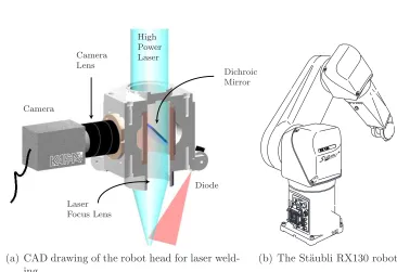
Camera
Camera Lens
High Power Laser
Diode
Laser Focus Lens
Dichroic Mirror
(a) CAD drawing of the robot head for laser weld-ing
RX 130 R
0
65
XAM A1
oJc
aPM 6.0
P1
P2
aPM 6.0
(b) The St¨aubli RX130 robot
Figure 1.1: The robot and the laser welding head
The designed head (Figure 1.1(a)) contains a dichroic mirror, which reflects an image of the workpiece to a video camera while letting high power laser light pass through. The benefit of this setup is that the working point is always in the camera view. A disadvantage is that the image passes the laser focus lens, which has not been optimised for imaging purposes, but for a well focussed laser bundle. Because a large field of view is desired, not only the relatively distortion-free centre but also the outer parts of the laser focus lens will need to be used. This introduces large errors in the image, such as aberrations, radial distortions and coma (for explanations of these terms, please refer to [4, 5]). In Chapter 2 a procedure will be presented for determination and compensation of several camera and lens distortions. Chapter 3 deals with the results of experiments using this procedure.
1.2 RESEARCH OVERVIEW 5
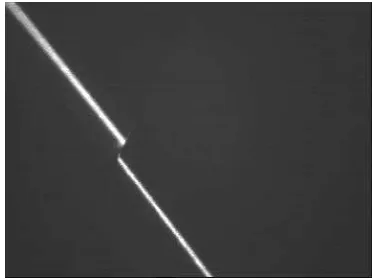
known. To determine this distance, laser diodes attached to the welding head will project lines onto the surface of the workpiece (see Figure 1.2(a)). The posi-tion of the projected lines in the images provides informaposi-tion about the posiposi-tion and orientation of the welding head relative to the workpiece. The fixed relation between the camera and the light planes created by the laser diodes makes it pos-sible to calculate this position and orientation. This is called triangulation. For an overlap joint the seam itself usually appears as a break in the line projection, as can be seen from Figure 1.2(b). Chapter 4 elaborates on triangulation and the determination of the seam position and experimental results are presented in Chapter 5.
The head is attached to a St¨aubli RX130 robot (Figure 1.1(b)) of which the dynamical behaviour is thoroughly examined by other research groups within the mechanical automation laboratory. A calibration of the tool – which in-cludes the determination of the laser focus point relative to the robot tip and the determination of a pixels-to-millimetres scaling – is described in §4.4.
(a) A laser diode projects a line on the seam, which is viewed by a camera positioned un-der a known relative angle
(b) The camera image shows broken lines in case of projection over an overlap joint
Figure 1.2: The principle of triangulation
Chapter 2
Image Undistortion
Almost all images we see are distorted somehow. Especially when lenses are used distortions become clearly visible. This can be seen when you put on somebody else’s glasses, when you look through a peep hole or fish eye in the door, or when you are close to a webcam. Professional camera lenses are optimised to minimise these effects, but small, cheap lenses or lenses designed for purposes other than imaging (such as the laser focus lens in the integrated welding head) often suffer from severe distortions.
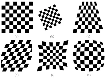
(a) (b) (c)
(d) (e) (f)
Figure 2.1: Several transformations: (a) Original
(b) Linear Conformal (c) Projective / Perspective (d) Affine / Skew
(e) Radial: Pincushion
2.1
Introduction to Distortions and Calibration
Several transformations occur when a 2D image is taken of a 3D scene. Rotation and perspective (Figures 2.1(b)–(c)) for instance depend on the viewpoint relative to the scene. Skew, pincushion and barrel transformations (Figures 2.2(d)–(f)) on the other hand, depend on the optics and camera properties. Scaling depends on both.
Here we will adopt the definition of ‘distortion’ given by Merriam-Webster’s dictionary[6]: a lack of proportionality in an image resulting from defects in the
optical system. This rules out the viewpoint-dependent transformations, because
they do not originate in the optical system. It also rules out spherical aberrations and astigmatism, because they do not introduce a lack of proportionality in the image, but only a blurring effect.
2.1.1
Problems Due to Distortions
The main distortions in an image are radial distortions, where pixels are moved from or towards the optical centre with an amount related to their distance from this centre. Radial distortions cause straight line(s) in the real world to be displayed as a curve in the camera image, as Figure 2.2(a) shows. Fitting a straight line through a curve will result in inaccurate results, as the fitted line will always deviate from the line in the image at several places.
Another problem occurring due to radial distortions, is that two objects in the centre of the image may be 10 pixels apart, whereas two other objects, equally distant in the real world, may appear 15 pixels apart when positioned at the edge of the image. Figure 2.1(e) illustrates this: the once equally sized squares of figure Figure 2.1(a) appear larger at the image edges after distortion. This means a line at the edge is not only curved, it will also be shifted.
It is therefore important correct any radial distortions in the images, before any feature extraction – such as seam detection – is done.
(a) The distorted image shows curved lines, which are difficult to fit accurately.
(b) After the images is undistorted, the lines are straight again which makes accurate fitting possible.
2.1 INTRODUCTION TO DISTORTIONS AND CALIBRATION 9
2.1.2
Projective Geometry
To determine the influence of distortions on the image, some basic knowledge about image projections is needed. When relating features in images to the real world, a transformation between the 2D image and the 3D world must be defined. The camera model used here is that of a pinhole camera[7]. This widely used model is simple yet powerful and applicable to most off-the-shelf cameras. The pinhole camera is an extension of the perspective projection which gives the ideal transformation from a 3D point M = [x,y,z]T
to a 2D image point m = [u, v]T,
assuming that all light rays pass through a pinhole C (also called optical centre) at distance fc from the image plane.
C fc c
m M xc yc zc u v
Figure 2.3: Virtual image plane.
The perspective projection states that (see also Figure 2.3):
u
xc
= v
yc
= fc
zc
,
which can be rewritten to
zcu
fcxc
= zcv fcyc
,
or, in matrix-vector form withsset equal tozc by the lower row in the equation:
s u v 1 =
fc 0 0
0 fc 0
0 0 1
x y z c ,
or for short, using the augmented vector m˜ = [mT,1]T
sm˜ =FcMc
The perspective projection is extended with a camera transformation (see also Figure 2.4). This is needed because generally the camera image will not have its origin in the principal point c, but at some distance [u0, v0] from it. Also the size
of pixels in the image is in the extension, as the position of a point in the image is measured in pixels, rather than in millimetres. As the pixels need not to be square, different sizes for theudirection (ku) and v direction (kv) exist. The last
parameter is the angleθ, which specifies the perpendicularity of the image axes. Because these parameters specify the internal behaviour of the camera, they are called the cameraintrinsic parameters. The full pinhole camera model can now be written as:
Image Coordinates
Camera Coordinates
World Coordinates
C c = [u
0, v0]
fc
m M
θ
[R t]
x y z u v xc yc zc
Figure 2.4: Coordinate Systems in Projective Geometry.
s u v 1 =
ku kucotθ u0
0 kv/sinθ v0
0 0 1
fc 0 0
0 fc 0
0 0 1
x y z c =
fcku fckucotθ u0
0 fckv/sinθ v0
0 0 1
x y z c (2.2)
In this equation a change in the focal length fc – i.e., the distance between
the optical centre C and the principal point c – cannot be distinguished from a change in the pixel dimensions ku and kv. Therefore they are split in a slightly
different way, only for convenience: the zooming part of the camera intrinsic matrix, which is the upper-left 2×2 matrix, is normalised to be non-magnifying:
s u v 1 =
α γ u0
0 β v0
0 0 1
f 0 0
0 f 0
0 0 1
x y z c
or for short
2.1 INTRODUCTION TO DISTORTIONS AND CALIBRATION 11 With: α γ 0 β f ro
=√2 (2.4)
and thus: f =
fcku fckucotθ
0 fckv/sinθ
f ro √ 2 (2.5)
Using Equation 2.3 a point expressed in the camera coordinate system can be projected onto the image plane. In practice the position of a point is not known with respect to the camera, but only with respect to a world coordinate system. This system can be rotated and translated with respect to the camera, as shown in Figure 2.4. A 3×3 rotation matrix R and a translation vector
t= [∆x,∆y,∆z]T describe the transformation:
Mc =RM+t,
or, written out in full:
x y z c =
r11 r12 r13
r21 r22 r23
r31 r32 r33
x y z + ∆x ∆y ∆z ,
which can be written using an augmented vector as
=
r11 r12 r13 ∆x
r21 r22 r23 ∆y
r31 r32 r33 ∆z
x y z 1 , or
Mc = [R t]~M.
(2.6)
Because the transformation [R t] takes place outside the camera, R and t are called the camera extrinsic parameters.
The full transformation from a 3D model, expressed in world coordinates to a 2D images can be written by combining Equations 2.3 and 2.6 to:
sm˜ =AF[R t]~M. (2.7)
Special Case for a 2D Model
of the world coordinate system1. This results in
sm˜ =AF
r11 r12 r13 ∆x
r21 r22 r23 ∆y
r31 r32 r33 ∆z
x y 0 1 =AF
r11 r12 ∆x
r21 r22 ∆y
r31 r32 ∆z
x y 1 (2.8)
By abuse of notation, for the rest of the report ~M is redefined to x y 1T
instead of x y z 1T. The transformation matrices are gathered into the homographyHwhich thus relates the real world point (or model point)Mto the image pointm:
sm˜ =AF[r1 r2 t]
| {z }
HomographyH
~
M. (2.9)
2.1.3
Calibration
To compensate the distortions, the parameters of the camera and optical system must be known. Calibration is the art of finding these parameters. For the camera the intrinsic parameters (§2.1.2, Equation 2.3) will need to be determined and for the radial distortions two extra parameters have to be found. When these parameters are known, they can be used to undo images taken with that camera from distortions.
Most camera calibration procedures make use of a pattern of regularly spaced objects. These objects can for instance be points, lines or squares (see Figure 2.5). Multiple pictures of the pattern are taken under different angles. The main goal is then to find a ‘common factor’ in all images, to distinguish between the camera (varying) extrinsic parameters (§2.1.2, Equation 2.6) on the one side and the (constant) intrinsic parameters and distortions on the other side.
A model describes the positions of the objects in the pattern based on fea-tures (‘keypoints’) that can later be detected in the images (such as a centroid, crossings or corners). The parameters can be found by fitting the keypoints ex-tracted from the images to the mathematically transformed and distorted model positions. Most procedures (like those of Tsai[8, 9], Heikkila[10] and Savii[11]) require a model containing the absolute 3D position of calibration points, or well defined relative movements between two calibration images. Zhang’s method [1] however, is flexible and only needs relative 2D positions of a 2D pattern for the model points. This is why Zhang’s method was chosen for camera and lens calibration2.
1 It could be assumed that the model exists at x= 0 ory= 0 instead.
2 After implementation it appeared that Zhang’s method was found to have the best (but
2.1 INTRODUCTION TO DISTORTIONS AND CALIBRATION 13
(a) (b) (c)
(d) (e)
Figure 2.5: Common calibration patterns:
(a) The checkerboard image used for the Matlab Camera Calibration Toolbox [13] (b) The pattern used by Zhang [1]
(c) The pattern used for the Halcon software [14] (d) 3D grid as used by Heikkila [10]
(e) 3D grid with lines as used by Jong-Eun Haa & Dong-Joong Kangb [15]
A Step-by-Step Guide for Calibration
The rest of this chapter will deal with all aspects of camera and lens calibra-tion and image undistorcalibra-tion in a chronological way. Calibracalibra-tion consists of the following steps, with step 3 in accordance with Zhang:
1. Preparation of a calibration pattern (typically black squares on a white background) and taking pictures of it with the system to be calibrated
2. Extraction of the keypoints for every image, i.e., the extraction of char-acteristic points in the image that can be matched with a model of the calibration pattern
(a) Identification of the keypoints (determination the location of the key-points, e.g., centroids or corners of the black squares)
(b) Ordering of the keypoints, to make sure the list of keypoint coordinates has the same order as the list in the model definition)
3. Estimation of the camera and lens distortion parameters from a set of images
(b) Estimation of the camera intrinsic parameters (the common part in all images) and extrinsic parameters (rotation, translation)
(c) Calculation of the radial distortion parameters based on all images. This is implemented by a least squares optimisation to determine which distortion parameters describe the transformation Model→ Im-age best
(d) Refinement of all estimates. Because the radial distortion parameters are estimated upon estimations of in- and extrinsic parameters that are not corrected for this distortion, an (iterative) refinement should be carried out.
After the calibration is done and the camera and lens parameters are known, images can be undistorted. The undistortion procedure is described in §2.5.
2.2
Calibration Pattern & Image Acquisition
When using clearly separated objects like in Figures 2.5(b) and (c) it is easier to find the keypoints than when using a checkerboard-like model (Figure 2.5(a)). A pattern with objects ordered in equally spaced rows and columns is preferred for convenient ordering. Although Zhang uses the corners of the black squares as keypoints, here the centroids of the objects will be used. A detailed explanation and a justification for this choice can be found in §B.13.
The theoretical minimum number of images required is 3, but it is preferred to take 10-20 images depending on the image quality. It is important to keep the optical system fixed and equal to the settings that will be used later on, when images need to be undistorted. This is because the parameters estimated in the calibration process will be different for different lenses and camera settings such as focus distance and aperture.
2.3
Keypoint Extraction
Finding the keypoints actually consists of two steps: identifying their locations and placing them in the right order. It is important to have the order of the keypoints list (e.g. bottom to top, then left to right) equal to the order of the model, because otherwise a least squares fit of (distorted) model points to the keypoints would not make any sense.
2.3.1
Keypoint Identification
The first step in identification of the keypoints is identification of the objects. Objects can be identified by thresholding (§A.2) and labelling (§A.3) the image. From the labelled objects, the keypoints can be derived easily.
2.3 KEYPOINT EXTRACTION 15
Thresholding the images is not trivial. Several problems occur, varying from in-homogeneous lighting to coma effects caused by the laser focus lens and internal reflections originating from the semi transparent mirror. Multiple thresholding algorithms have been implemented to suit the needs for different kinds of im-ages. Appendices C.1 and C.2 deal with these algorithms and their suitability for different image types.
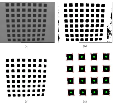
When a black/white image (Figure 2.6(b)) is available, each set of intercon-nected black pixels should be identified as an object, and the centroid of this object should be determined. When labelling the image it is important to keep in mind that only the calibration objects should be labelled. Therefore, after thresholding all objects that are not calibration objects must be removed (Fig-ure 2.6(c)). Most of these unwanted objects can be ruled out by examining their size (often they originate from noise and thus are much smaller) or position (the image edges are usually a source of unwanted objects). The minimal size for an object to be recognised as a calibration object is set depending on the image size, the number of objects and the number of black pixels in the image.
After all calibration objects have been identified, the keypoints can be cal-culated. For the centroids this normally means that all x-coordinates of the pixels that are forming the object are averaged and the same is done for all y-coordinates (Figure 2.6(d)), however in Appendix C.3 a more advanced method is proposed.
The corner keypoints are determined using the following strategy: the first keypoint is the position of the pixel which is the furthest away from the centroid. The second keypoint is the position of the pixel second furthest away from the centroid, ignoring all pixels within a given distance4 from the keypoint already
found. This process goes on until all corners of the object are found. With the correct setting of the distance for ignoring pixels, this method appears quite robust.
2.3.2
Keypoint Ordering
It is important to have a convention for the order of the keypoints. How they are ordered is not important, as long as the model and the extracted points can be matched. We decided to order first from low to high vertical coordinates and then from low to high horizontal coordinates. This does not necessarily match with bottom-top and x and y coordinates, because images pixels are often described in a differently positioned coordinate system.
Although we humans can find the right order of points with ease, it is quite difficult to make this clear to a computer in an unambiguous way. First of all the computer must know which objects are on the corners of our calibration pattern. The first step is to determine the so-called convex Hull, which finds the outermost objects in the set, i.e. all points that would be touched by a rubber band wrapped around the set, as depicted in Figure 2.7(a). To find out which of these points
4 This distance is calculated from the minimum object size, which in its turn is based on the
(a) (b)
(c) (d)
Figure 2.6: Identification of keypoints: (a) The original image
(b) The thresholded image
(c) The thresholded image, cleaned from unwanted objects
2.3 KEYPOINT EXTRACTION 17
are on the corners, the angles between the lines with neighbouring points are investigated. The four largest angles (closest to 90 degrees) are assumed to correspond to the corner objects.
Now we know all corner objects, we can select the two with the lowest hori-zontal coordinate and from that selection we pick the one with the lowest vertical coordinate (see also Figure 2.7). This is our starting point.
1 2 3 4 5 6 7 8 (a) 1 2 3 4 5 6 7 8 (b) 1 2 3 4 5 6 7 8 (c)
Figure 2.7: The convex hull transform is used to determine the starting point for keypoint ordering
(a) The convex hull selects all points touched when a rubber band would be wrapped around a set. The corner objects can be found by examining the angles the interconnecting lines make: the lines 8–1 and 1–2 make an angle of approximately 90◦ and the lines 2–3 and 3–4 make an angle of almost 0◦, so
1 is a corner object and 3 is not.
(b) Of the 4 corner objects, the ones with lowest horizontal index are taken (8 and 1)
(c) Of the 2 remaining corner objects, the one with lowest vertical index is taken (1)
Finding the next object works as following (see also Figures 2.8 and 2.9):
1. Find the 5 objects closest to the current one (3 when starting a new column)
2. Of these 5, select those that have a higher vertical coordinate than the current object
3. Of these, select the 2 leftmost objects
4. Determine the angle between the vectors from the current object to the 2 candidates
5. If the angle is small (Figure 2.8(c)), take the closest object, else take the leftmost (Figure 2.9(c))
(a) Step 1 (b) Step 2 (c) Step 3–5
Figure 2.8: Determining which is the next keypoint, scenario 1. The encircled point is the current point, the point with the square will be the next point.
(a) Step 1 (b) Step 2 (c) Step 3–5
2.4 CAMERA AND LENS DISTORTION ESTIMATION 19
For the ordering of corner keypoints the convex Hull is used again, as it always orders points counter-clockwise. The only thing that remains to be done is to find out which of the four points comes first. Of the two points with the lowest horizontal coordinate, this will always be the one with the lowest vertical coordinate. Figure 2.10(b) shows the resulting order.
(a) Order of the centroid keypoints, regard-less of object shape.
(b) Order of the corner keypoints, for square objects.
Figure 2.10: Pattern keypoint order.
2.4
Camera and Lens Distortion Estimation
To be able to estimate the lens distortions, the perspective distortions must be eliminated. Therefore the first step is to find a linear transformation matrix that matches the extracted sets of keypoints to the calibration model. From these homography matrices (one for each image), the intrinsic (camera specific) and extrinsic (orientation specific) parameters can be extracted. Then the radial distortions can be estimated.
Both model points M and the keypoints m are normalised to improve matrix conditions. The model points are transformed such that their centre of gravity is at the origin and their mean distance to the origin is √2, so a typical point will look like [x,y] = [1,1]. The keypoints are normalised in almost the same way, but their origin and scaling are determined upon all pixels in an image, instead of on the keypoints themselves. This is because the image provides constant and easily reproducible factors, so the scaling is the same in all images and can be re-calculated any time, as long as the image dimensions are known.
2.4.1
Finding the Homography
Recalling Equation 2.9 from §2.1.2 we know that in the ideal case
sm˜ =H~M with: H=AF[r1 r2 t], (2.10)
it contains both the intrinsic and extrinsic parameters, a homography must be estimated for each image of the model plane.
Equation 2.10 can also be written as
su= ¯h1~M (2.11)
sv = ¯h2~M (2.12)
s= ¯h3~M, (2.13)
or
0 = ¯h1~M−u¯h3~M (2.14)
0 = ¯h2~M−v¯h3~M, (2.15)
(2.16)
which makes it easier to put in a matrix-vector form
~
MT 0 −un~MT
0 ~MT −v n~MT
| {z }
L ¯ hT 1/η ¯ hT 2/η ¯ hT 3
| {z }
x =0 where: sc= √ 2 n n X i=1 kmik
un=
u
η, vn = v η
(2.17)
to determine a least squares solution for H, which is needed as an initial guess for the non-linear least squares optimisation. The solutionxin the least squares sense is known to be the eigenvector corresponding to the smallest eigenvalue of
LTL. This calculation has been optimised using the extra normalisation factor
η.
Using the initial guess as starting point a non-linear optimisation is per-formed: minH
P
ikm˜ −H~M/sk
2
and an accurate homography is found for each image. The homography is always normalised afterward such that h33 = 1
be-cause the scaling-factor s is present in Equation 2.10 anyway.
2.4.2
Camera Intrinsic & Extrinsic Parameter Estimation
The homographies should be split into two parts: the intrinsic parametersAand
2.4 CAMERA AND LENS DISTORTION ESTIMATION 21
Using the fact that5
h1 h2 h3
=λAFr1 r2 t
, (2.18)
the orthonormality of the rotation matrix can be rewritten to:
rT1r2 = 0 ⇒ hT1(AF)−T
1
λ
1
λ(AF)
−1h 2 = 0,
rT1r1 = 1 ⇒ hT1(AF)
−T(AF)−1h
1 =λ2,
rT2r2 = 1 ⇒ hT1(AF)
−T(AF)−1h
2 =λ2,
(2.19)
so the following must hold:
hT1(AF)−T(AF)−1h2 = 0,
hT1(AF)−T(AF)−1h1 =hT2(AF)
−T(AF)−1h 2.
(2.20)
The fact that there are only 2 constraints per image, means that at least 3 images are needed to determine the 5 degrees of freedom6 in AF. Now let
B= (AF)−T(AF)−1 =
B11 B12 B13
B12 B22 B23
B13 B23 B33
= 1
f2α2 −
γ f2α2β
γ v0−β u0 f2α2β
−f2γ α2
β
γ2 f2
α2 β2 +
1
f2
β2 −
γ(γ v0−β u0) f2
α2
β2 −
v0 f2
β2
γ v0−β u0 f2
α2
β −
γ(γ v0−β u0) f2
α2
β2 −
v0 f2
β2
(γ v0−β u0)2 f2
α2
β2 +
v02 f2
β2 + 1
, (2.21)
then, to write the orthonormality equations (Equation 2.20) in a homogeneous matrix-vector form, we write
vTijb=hTiBhj, (2.22)
with:
b= B11 B12 B22 B13 B23 B33
, (2.23)
and thus:
vij =
hi1hj1
hi1hj2+hi2hj1
hi2hj2
hi3hj1+hi1hj3
hi3hj2+hi2hj3
hi3hj3 . (2.24)
5 Theλwas introduced becauseHhas been defined upon a scale factor. 6 These 5 degrees of freedom are the parametersα, β, γ, u
0, v0andf with the normalisation
This way we obtain the constraints in matrix-vector form for every image:
vT
12
(v11−v22)T
b=0. (2.25)
When we do this for all of the n images, we get a matrix V with dimensions 2n×6. b can be solved up to a scale factor λ by calculating the eigenvector corresponding to the smallest eigenvalue of VTV. From this vector b we can
extract the parameters inAF as following:
v0 = (B12B13−B11B23)/ B11B22−B212
,
Λ =B33− B132 +v0(B12B13−B11B23)
/B11,
αf =pΛ/B11,
βf =
q
ΛB11/(B11B22−B122 ),
γf =−B12(αf)2βf /Λ,
u0 =γv0/β−B13(αf)2/Λ,
f = √1 2 αf γf 0 βf f ro . (2.26)
Once the parameters contained in AF are known, the extrinsic parameters
R and tcan be calculated from Equation 2.18 using
λ= 1/k(AF)−1h
1k= 1/k(AF)−1h2k
r1 =λ(AF)−1h1
r2 =λ(AF)−1h2
r3 =r1×r2
t=λ(AF)−1h3.
(2.27)
However the obtained rotation matrix R = r1 r2 t
is not guaranteed to be orthonormal, due to noise on the keypoint positions. As Zhang states in Appendix C of [1], the singular value decompositionUSVT =R can be used to fit a proper rotation matrixRnew to the calculated R. According to Zhang this
new rotation matrix would be Rnew = UVT, but actually the determinant of
Rnew should still be checked, because if it is −1 the matrix is mirroring as well.
In that case Rnew=−UVT should be used.
2.4.3
Radial Distortion Parameter Estimation
2.5 IMAGES UNDISTORTION 23
For undistortion only the non-magnifying camera matrixAand the distortion factors are needed. Therefore the zooming F and extrinsic transformations (ro-tation and translation) should already be applied to the model points before the distortions are added. The distorted image points are therefore calculated from the normalised model keypoints in camera coordinates [x,y,z]T
c,n, pre-multiplied
with the zooming matrix. The radial distortions can be described using78
˘
u=u+ (u−u0)
h
κ1 x2+y2
+κ2 x2+y2
2i
(2.28)
˘
v =v+ (v−v0)
h
κ1 x2+y2
+κ2 x2+y2
2i
, (2.29)
whereκ1 and κ2 are the radial distortion parameters. Now for every keypoint in
every image we can write
(u−u0) (x2+y2) (u−u0) (x2+y2) 2
(v −v0) (x2+y2) (v−v0) (x2+y2)2
κ1 κ2 = ˘
u−u
˘
v−v
. (2.30)
If we stack all these equations we can find the values for κ1 and κ2 in the
least-squares sense using the pseudoinverse (see also §B.2).
2.4.4
Solution Refinement
All parameters have been determined now. However, the homography, rotation matrix and translation vector and camera intrinsic parameters were determined under the assumption that there were no distortions. This means that these estimates are inaccurate and thus the calculated radial distortions will be as well. An iterative process could lead to an optimal estimation of all parameters, but according to Zhang, a non-linear least-squares optimisation taking into account all parameters at the same time performs better.
The optimised parameter values will be calculated by the minimisation of
n X i=1 m X j=1
kmij−m˘(A, κ1, κ2,Ri,ti),Mjk2 (2.31)
using the Levenberg-Marquardt routine[19], with the previously calculated pa-rameter values as initial guess. To reduce the number of papa-rameters to optimise and to make sure an unconstrained optimisation can be carried out, the rotation matrices will be exchanged by Rodrigues parameters. Rodrigues’ formula (§B.3) can be used to describe a rotation with the absolute minimum of 3 parameters and provides easy conversion from and to the original 3×3 rotation matrix.
2.5
Images Undistortion
Most procedures to undo images from their distortions somehow use the inverse of the distortion function. For the distortion functions used here (Equation 2.29)
according to literature this would mean that an iterative process is needed. Other researches have focussed on developing distortion functions that can easily be inverted[17].
All these efforts seem unnecessary if we realise that we can just distort an ‘empty’ destination image, see where the pixels would go, and extract the image data at these positions from the (distorted) source image. Actually the functions used for translating model points in camera coordinates to distorted image points (Eqs. 2.28 and 2.29) are used again, but now with the coordinates of all pixels instead of the keypoints. This procedure is illustrated by figure 2.11.
This newly developed technique is practical, accurate and fast, but for a real-time implementation things can be speeded up even more. A file with undistor-tion parameter values is read upon the program start-up and a lookup-table is created defining for every point in the undistorted image, from which pixel in the distorted image the intensity should be taken. In real-time, the only thing that needs to be done is to apply the lookup-table to transform the image pix-els, which is very fast. Interpolation could be done, but this will slow down the undistortion process.
Chapter 3
Camera Calibration Experiments
A number of experiments have been carried out to test the camera calibration strategy discussed in Chapter 2. The image processing and keypoint extraction appeared to be quite sensitive to the quality of the images provided. Both ‘good’ and ‘bad’ quality images1 were used in separate tests to verify performance on
the one hand and practical applicability on the other hand.
3.1
Introduction
Many series of images have been captured and processed in various ways. In the evaluation of the results several methods were used to measure the performance of the estimated parameters in undistortion. Analysis techniques have been de-veloped and settings have been tuned during the testing phase. Where possible, old results have been re-analysed with new settings to improve comparability.
3.1.1
Overview of Experiments
The experiments covered in this chapter are:
• Experiments on keypoint extraction, in §3.2
• Calibration based on simulated data sets and images, in §3.3
• A comparison with the results obtained by Zhang, in§3.4
• Calibration of a photo camera, in §3.5
• Calibration of the optical system in the laser welding head, in §3.6
The tests in general were carried out in the following way:
1. 10–25 Images are taken and their keypoints are extracted
2. Image subsets are made (usually consisting of 4 images)
3. All subsets are fed to the calibration algorithm (when many subsets are available, the total number is mostly limited to 2000–3000 sets)
4. The results are processed:
(a) The average number of refinement iterations is calculated per image (b) The average and standard deviation of all subset results are calculated
for every estimated parameter
(c) The average and standard deviation of the subsets with lowest RMS (see §B.4) are calculated for every estimated parameter
(d) The averaged results forall and for thelowest RMS subsets are saved separately for use with the undistortion algorithm.
3.1.2
Performance Standards
Several performance standards have been applied to measure the quality of a pa-rameter set resulting from the calibration routine.Where possible the outcomes were related to known reference values, otherwise a visual or mathematical analy-sis was made of images undistorted with the calculated parameters.
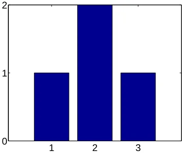
Histograms
The results of all subsets are compared with each other by calculating the aver-ages and standard deviation over the subsets for every parameter (§3.1.1). To visualise these results, histograms have been plot. The example in Figure 3.1 shows a histogram for a set results like [2, 1, 3, 2]. The resulting values are on the horizontal axis and their frequency of occurrence is on the vertical axis. This means that the bar at 2 has height 2, because it is twice in the set of results, whereas the bars at 1 and 3 have height 1.
In the histograms throughout this chapter, the vertical axis has been nor-malised. This has been done because the different optimisations have different numbers of subsets. The ideal histogram is supposed to show a sharp peak (with normalised height 1) at the actual parameter value.
Analysis of Undistorted Images
In the end the estimated parameters should result in a proper undistortion of images. To test this the original images were undistorted using the parameters found by calibration. Keypoints were extracted from the undistorted images and horizontal and vertical lines were fit through the keypoints. The residual of the fit was used as a measure to compare the quality of different estimates.
3.2 KEYPOINT EXTRACTION 27
1 2 3
0 1 2
Figure 3.1: Example histogram of a set experiments resulting in a value 1 once, 2 twice and 3 once.
Note:
Most values in this chapter are the result of a normalised parameter optimisation. This means that the values do not immediately represent a physical quantity. The values are used in this normalised form for undistortion as well, which makes a comparison of these values more sensible than one of the un-normalised values.
3.2
Keypoint Extraction
Several thresholding algorithms were implemented to be able to process images of varying quality. Most of these are are result of testing different normalisation and thresholding strategies on images that were not thresholded satisfactory with any of the existing algorithms. Appendix C contains detailed information about the algorithms and their applicability.
In general it can be stated that only for qualitatively good images thresholding can be accurate enough to extract meaningful corner keypoints. This is because the corners are far more sensitive to inaccurate thresholding than centroids, as explained in §B.1.
For sharp images the keypoint extraction from a thresholded image works very good, even for corners. Figure 3.2(a) shows that on the images used by Zhang the proposed thresholding and keypoint extraction algorithms even perform better than the algorithms he uses (which have not been published).
(a) (b) (c) Figure 3.2: Determination of corner keypoints:
(a) cut-out of an image by Zhang, keypoints extracted after dynamic thresholding II (§C.2.2) depicted as stars, Zhang’s data (with software by Brian Guenter) as dots.
(b) cut-out of a thresholded image taken using the robot head, it is difficult to indicate where the corners are
(c) projection of the keypoints determined in (b) in the original image, determin-ing a proper threshold level is difficult, but critical
Labelling Problems
Some problems occurred due to labelling (§A.3) too many or too few objects. Objects connected to the border of the image and objects smaller than a certain size are neglected automatically, but sometimes an extra opening operation (ero-sion followed by dilation, see also§A.4) was needed to make sure that abusively thresholded parts in the background got connected to the edge. If calibration objects would have been poorly separated, a closing operation (dilation followed by erosion) could have been applied.
3.3
Simulations
For testing purposes several simulations have been carried out. Sets with key-points have been generated and images have been generated artificially to provide a controlled testing environment with known camera and lens errors and known rotations and translations. The details of the generation of these datasets and images can be found in§D.2.3.
3.3.1
Simulation Data
Non-normalised Data
3.3 SIMULATIONS 29
suffice when the parameters are normalised.
Estimates are very inaccurate and the spread in parameters found by analysis of different sets is large. When only the 10% results with the lowest RMS values are considered the results are quite well.
No Radial Distortions
Another test was carried out without radial distortions. A little random noise (about 0.1% of the image width) was added to the keypoint position data to pre-vent singularities in the calculation process. The parameter refinement converged in only 10 iterations, taking about 1.8 second per set. It could be expected that this converges faster than the other normalised tests (25 iterations), because the parameters estimated using the homograpy do not suffer from inaccuracies due to radial distortions, so they are already quite accurate.
The standard deviation of the parameters calculated from different sets of images are a lot smaller than in the other tests. The parameters are estimated accurately. Only the optical centre [u0, v0] is less accurate, probably because the
radial distortion enhances the effect of its location.
Different Noise Levels
Tests with increasing noise levels show an increasing variance in the results of the different image sets, as displayed in Figure 3.3. Especially the radial distortions appear difficult to estimate. The value for the first radial distortion parameter
κ1 is actually always wrong, probably because it is so small and its effect is
over-shadowed by the second order radial distortion.
0.980 0.982 0.984 0.986 0.988 0.99 0.992 0.994 0.996 0.998 1 20
40 60 80 100 120
(a) Without noise
0.98 0.982 0.984 0.986 0.988 0.99 0.992 0.994 0.996 0.998 1 0
20 40 60 80 100 120
(b) With 0.1% noise
0.980 0.982 0.984 0.986 0.988 0.99 0.992 0.994 0.996 0.998 1 20
40 60 80 100 120
(c) With 1% noise Figure 3.3: Histograms for the variable α.
Conclusions
• Normalisation saves a lot of time and improves accuracy,
• Taking the results from images sets with the 10% lowest RMS values highly improves accuracy,
3.3.2
Simulation Images
Keypoint OrderingFrom all generated test images, only for one the extracted keypoints could not be ordered properly. This image had huge radial and perspective distortions, which are very unlikely to occur in practice. Aside from this single image, the ordering algorithm has proven to be considerably robust.
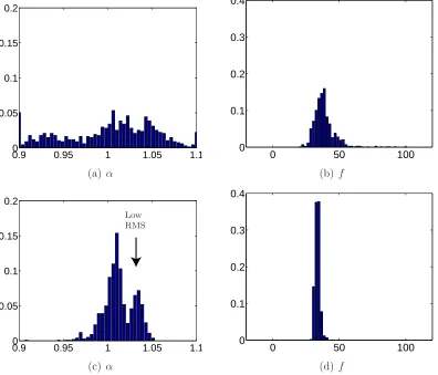
Varying the Number Of Images In a Subset and the Maximum Rota-tion Angles
Figures 3.4 and 3.5 show some of the results from 4 different tests. Figure 3.4 contains results from parameter estimations where images with small rotation angles (up to 5◦) were simulated. This means that perspective distortions are
relatively small. For the results in the left column subsets of 4 images were used to base the parameter estimation upon, for the right column subsets of 9 images were used. For Figure 3.5 large rotation angles (up to 45◦) were simulated. The
images at the left are for estimations with subsets of 4 again and the images at the right for subsets of 9 images.
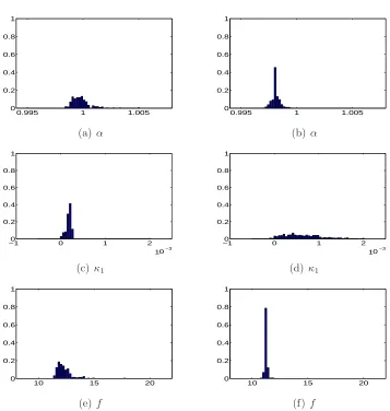
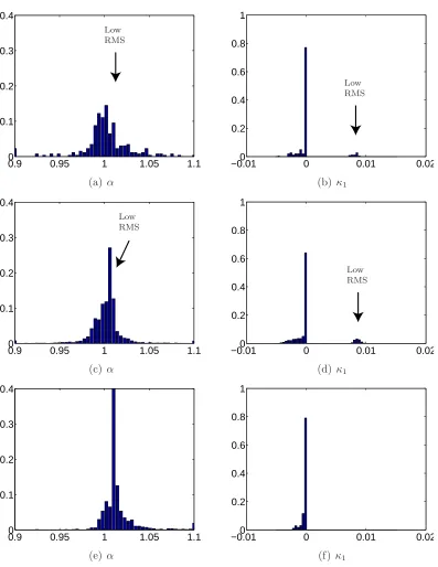
The first row of histograms in both figures shows the RMS value, which is a measure for the quality of the estimation. As a lower RMS indicates a higher quality, the estimates of the experiments with small angles seem to be better than those of the experiments with large angles. In all cases two or more peaks are visible. This indicates that there are local optima present in the optimisation space. For the other parameter histograms, peaks mainly incorporating results from sets in the low-RMS peak are indicated with an arrow whenever appropriate. For images with small rotations, it appears to be beneficial to use more images in a subset. The parameter estimations are clearly more stable when subsets of 9 images are used, then when 4 images are used. When only results with a low RMS are taken into account, the number of usable results is higher and the histograms show sharper peaks.
An Accurate Estimation of f
A problem however, is that the factor f is estimated totally wrong. As listed in§D.2.3, the value should be 40, whereas it is estimated somewhere between 5 and 20. This is probably due to the fact that the difference between the factor
f and the translation from and to the pattern ∆z (which is in t) have almost the same effect on an image. The only way to distinguish between them is by the perspective distortions, which are very small when only small rotations are present. Numeric results confirm the strong coupling of the estimated values of
f and ∆z.
For undistortion no accurate estimation of f is needed, as it is just a scaling from the model to the image. Actuallyf was extracted from the camera matrix
3.3 SIMULATIONS 31
used to relate image coordinates in pixels to real world coordinates in millimetres. Therefore simulations using images with large rotations have been done to try and find a more accurate value for f.
Figures 3.5(i) and (j) indeed show that with larger rotation angles (and thus larger perspective deformations) lead to a better estimate forf. Except for small improvements of u0 and v0, which can be estimated from both radial distortion
effects and perspective deformations, the other parameters however are estimated a lot worse: the histograms for α for instance (Figures 3.5(c) and (d)) are wide and the main peaks are at about 1.1 whereas they should be at 1.0094.
From the sharp peaks in Figures 3.5(e)–(h), one may think that the results forκ1 and κ2 have improved, but the opposite is true as the peaks are positioned
near 0 whereas they should be at 0.015 and 1·10−3 for κ
1 and κ2 respectively.
Only few results (the ones with low RMS) have an accurate value.
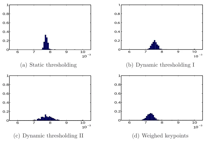
The Influence of Thresholding
The histograms in Figure 3.6 show the performance of some different thresholding techniques (these are discussed in detail in Appendix C). For these experiments images without radial distortions, but with blurring and light spots were used2.
Figure 3.6(a) shows that the (centroid) keypoints found from the static thresh-olding algorithm are not very consistent within an image, as the RMS values are quite high. The fact that the peak is relatively narrow indicates that the errors made in the different images are almost the same. The dynamic thresholding algorithms (Figures 3.6(b) and (c)) perform quite a bit better for some images, but the difference between images is larger. Weighed keypoint determination (Figure 3.6(d)) appears to find the most accurate positions for the keypoints for blurred images with non-homogeneous lighting.
Estimating Tangential Distortions
A test with tangential distortions, shows that it is very difficult to properly esti-mate the parameters when tangential distortions are present. The fact that the results are so poor, even with a perfectly matching model, is not very promising for real-life tests.
Conclusions
• Undistortion of images works, as Figure 3.7 shows,
• When using images with small rotation angles, using subsets of 9 instead of 4 images for parameter estimation gives more results that can be considered accurate,
• For an accurate estimation of the factor f large rotations are needed,
2 Images with radial distortion show the same tendency, although the RMS values are
con-siderably higher (8-9·10−3instead of 7-8·10−3) Images without blurring result in slightly
0 0.05 0.1 0 0.2 0.4 0.6 0.8 1 Low RMS (a) RMS
0 0.05 0.1
0 0.2 0.4 0.6 0.8 1 Low RMS (b) RMS
0.5 1 1.5
0 0.2 0.4 0.6 0.8 1 (c) α
0.5 1 1.5
0 0.2 0.4 0.6 0.8 1 (d) α
−0.01 0 0.01 0.02 0 0.2 0.4 0.6 0.8 1 Low RMS
(e) k1
−0.01 0 0.01 0.02 0 0.2 0.4 0.6 0.8 1 Low RMS
(f) k1
−1 0 1 2
10 0 0.2 0.4 0.6 0.8 1 3 − 10 Low RMS
(g) k2
−1 0 1 2
10−3 0 0.2 0.4 0.6 0.8 1 3 − 10 Low RMS
(h) k2
−200 0 20 40 60 80 100 0.2 0.4 0.6 0.8 1 (i) f
−200 0 20 40 60 80 100 0.2 0.4 0.6 0.8 1 (j)f
Figure 3.4: Overview of results for simulated images with relatively small rotations (c) (e) (g) (a) and (i) are results for subsets of 4 images,
3.3 SIMULATIONS 33
0 0.05 0.1
0 0.2 0.4 0.6 0.8 1 Low RMS (a) RMS
0 0.05 0.1
0 0.2 0.4 0.6 0.8 1 Low RMS (b) RMS
0.5 1 1.5
0 0.2 0.4 0.6 0.8 1 (c) α
0.5 1 1.5
0 0.2 0.4 0.6 0.8 1 (d)α
−0.01 0 0.01 0.02 0 0.2 0.4 0.6 0.8 1 Low RMS
(e) k1
−0.01 0 0.01 0.02 0 0.2 0.4 0.6 0.8 1 Low RMS
(f) k1
−1 0 1 2
10−3 0 0.2 0.4 0.6 0.8 1 3 − 10 Low RMS
(g) k2
−1 0 1 2
10−3 0 0.2 0.4 0.6 0.8 1 3 − 10 Low RMS
(h) k2
−200 0 20 40 60 80 100 0.2 0.4 0.6 0.8 1 (i)f
−200 0 20 40 60 80 100 0.2 0.4 0.6 0.8 1 (j) f
Figure 3.5: Overview of results for simulated images with relatively big rotations (c) (e) (g) (a) and (i) are results for subsets of 4 images,
6 7 8 9 10 10−3 0 0.2 0.4 0.6 0.8 1 3 − 10
(a) Static thresholding
6 7 8 9 10
10−3 0 0.2 0.4 0.6 0.8 1 3 − 10
(b) Dynamic thresholding I
6 7 8 9 10
10−3 0 0.2 0.4 0.6 0.8 1 3 − 10
(c) Dynamic thresholding II
6 7 8 9 10
10−3 0 0.2 0.4 0.6 0.8 1 3 − 10
(d) Weighed keypoints
Figure 3.6: Overview of the RMS values after parameter estimation based upon 4 simulated images without radial distortions, but with blurring and lights.
• Large rotations have a bad influence on the general quality of the parameter fits,
• A poorly estimated value for f does not influence undistortion, as it will be compensated for by a poor estimate of ∆z,
• The conclusion of the previous test, that taking the only results from im-age sets with the lowest RMS values highly improves accuracy, has been confirmed, as even in the test with big rotations the sets with low RMS provide good results,
• For blurred images with non-homogeneous lighting, the weighed keypoint determination gives the best keypoint locations,
• Estimation of tangential distortions should be refrained from, as calibration in that case does not provide meaningful values.
3.4
Zhang’s Test Images
The images and extracted corner keypoints Zhang uses to obtain the results pre-sented in his paper[1] are available from his website. These files have been used to verify the results of theMatlab implementation with the ones stated in the
3.4 ZHANG’S TEST IMAGES 35
(a) Original (b) Undistorted Figure 3.7: Undistortion of a simulated image.
3.4.1
Zhang’s Test Data
The keypoint data provided by Zhang were fed to theMatlabcamera calibration
program. To compare the output of the program (Table 3.1) to the results Zhang presents in his paper (Table 3.2), the values in Table 3.1 were un-normalised and compensated for taking the factor f out of the camera matrix AF.
quadruple (1234) (1235) (1245) (1345) (2345) mean st.dev.
α 832.289 836.402 836.380 834.087 836.525 835.137 1.890
β 832.289 836.402 836.547 834.253 836.525 835.203 1.896
γ 0.250 0.167 0.167 0.250 0.167 0.200 0.045
u0 304.924 303.869 302.662 304.175 303.013 303.729 0.908
v0 204.864 204.100 208.503 205.690 205.354 205.702 1.676
κ1 -0.246 -0.221 -0.227 -0.223 -0.222 -0.228 0.010
κ2 0.263 0.179 0.179 0.177 0.179 0.196 0.038
RMS 0.719 0.719 0.535 0.719 0.673 0.673 0.079
Table 3.1: Parameter estimates for several subsets of 4 images out of 5 using the
Matlabcamera calibration program.
Table 3.3 shows the difference in the results, where 1.00 means that there is no difference and 2.00 would mean that the value found using the Matlab
implementation is twice as big as the value Zhang reports. Although most values are almost equal, some differences are remarkable.
The differences in the variable γ – which is the skew factor in the images – can be explained by the fact that the standard deviations are about a quarter of the mean values (see Tables 3.1 and 3.2), which indicates that it is hard to estimate this variable correctly. The facts that the skew is very small (less than 0.01◦) and that perspective may result in a similar effect may play a role in this.
The difference in the RMS (Root Mean Square) values is hard to explain. Because the factor is always about 2 some difference in the calculation may exist3. On the other hand it could also mean that theMatlaboptimisation did
quadruple (1234) (1235) (1245) (1345) (2345) mean st.dev.
α 831.810 832.090 837.530 829.690 833.140 832.850 2.900
β 831.820 832.100 837.530 829.910 833.110 832.900 2.840
γ 0.287 0.107 0.061 0.136 0.110 0.140 0.086
u0 304.530 304.320 304.570 303.950 303.530 304.180 0.440
v0 206.790 206.230 207.300 207.160 206.330 206.760 0.480
κ1 -0.229 -0.228 -0.230 -0.227 -0.229 -0.229 0.001
κ2 0.195 0.191 0.193 0.179 0.190 0.190 0.006
RMS 0.361 0.357 0.262 0.358 0.334 0.334 0.040
Table 3.2: Parameter estimates obtained by Zhang.
quadruple (1234) (1235) (1245) (1345) (2345) mean st.dev.
α 1.00 1.01 1.00 1.01 1.00 1.00 0.65
β 1.00 1.01 1.00 1.01 1.00 1.00 0.67
γ 0.87 1.56 2.74 1.84 1.53 1.43 0.53
u0 1.00 1.00 0.99 1.00 1.00 1.00 2.06
v0 0.99 0.99 1.01 0.99 1.00 0.99 3.49
κ1 1.07 0.97 0.99 0.98 0.97 1.00 10.37
κ2 1.35 0.94 0.93 0.99 0.94 1.03 6.32
RMS 1.99 2.01 2.04 2.01 2.01 2.01 1.99
Table 3.3: Results of the Matlab implementation divided by the results listed in
Zhang’s paper.
not converge properly, however stricter convergence criteria did not make much difference.
The difference in standard deviations is remarkable, as the first 3 parame-ters, α, β and γ are twice as stable, but the other parameters are varying more. The most likely cause is the fact that the factor f was taken out of the cam-era matrix AF. A more sophisticated convergence criterion for the parameter refinement (§2.4.4) might improve the reliability of the estimates4.
Conclusions
• The Matlabimplementation works properly,
• Taking the zoom factorf out of the camera matrixAFslightly affects the standard deviation in results from different image sets.
while in theMatlab implementation the errordistance was used.
4 Foru
0 andv0the difference in definition (with respect to the upper left corner for Zhang
and to the image centre for the Matlab implementation) may also influence accuracy
3.5 PHOTO CAMERA CALIBRATION 37
3.4.2
Zhang’s Test Images
Using the images Zhang provides means that the keypoints should still be de-tected. Because the images provided are of good quality, there should not be much difficulty in finding the keypoints. As mentioned in §3.2 the detected cor-ners appear to be even more accurate than Zhang’s data when judged by eye.
To have a measure for the undistortion quality, horizontal and vertical lines were fit through extracted keypoints. The lower the norm of residuals summed over all fitted lines, the smaller the distortions are considered to be. A compen-sation was done for the fact that calculations with corner keypoints will have twice as many lines as those with centroid keypoints and that there will be twice as many points on each line.
The undistorted images have a total residual of about 300 pixels when corner keypoints are fitted and about 150 pixels when centroids are fitted. This differ-ence can be explained by the fact that corners are harder to detect accurately as discussed in§B.1. Another point is that the centroids are an average over the whole object and thus take less extreme values than the corner keypoints.
After undistortion the residuals are around 160 and 30 pixels for measure-men