R E S E A R C H
Open Access
Classification by diagnosing all absorption
features (CDAF) for the most abundant minerals
in airborne hyperspectral images
Mohammad Reza Mobasheri
*and Mohsen Ghamary-Asl
Abstract
Imaging through hyperspectral technology is a powerful tool that can be used to spectrally identify and spatially map materials based on their specific absorption characteristics in electromagnetic spectrum. A robust method called Tetracorder has shown its effectiveness at material identification and mapping, using a set of algorithms within an expert system decision-making framework. In this study, using some stages of Tetracorder, a technique called classification by diagnosing all absorption features (CDAF) is introduced. This technique enables one to assign a class to the most abundant mineral in each pixel with high accuracy. The technique is based on the derivation of information from reflectance spectra of the image. This can be done through extraction of spectral absorption features of any minerals from their respected laboratory-measured reflectance spectra, and comparing it with those extracted from the pixels in the image. The CDAF technique has been executed on the AVIRIS image where the results show an overall accuracy of better than 96%.
Keywords:remote sensing, hyperspectral, minerals, classification, absorption features
1. Introduction
The image classifications are based entirely on the spec-tral signatures of the land cover types. This area of spe-cialty has attracted the attention of remote sensing researchers in recent years and as a result, the techni-ques of classification have been improved considerably. These techniques have been divided into two general categories: supervised and unsupervised. In supervised classification, usually the statistical methods [1] and training samples are being used, whereas the unsuper-vised classification is based on the comparison between spectral signatures of a pixel and those of different materials collected in spectral libraries [2].
Spectral characteristics is a tool that has been used for decades to identify, understand, and quantify solid, liquid, or gaseous materials, especially in the laboratory. This is usually done through detection of absorption features due to the presence of specific chemical bonds, where its depth of absorption represents the abundance and physical state of the detected absorbing species
[3-5]. Imaging spectroradiometer can acquire data with suitable spectral range, resolution, and sampling rate at every pixel in a raster image, so that individual absorp-tion features can be identified and spatially mapped [6].
One of the most powerful methods in unsupervised classification is Tetracorder introduced by Clark et al. [7]. There are five innovations in this method where two of these are used in this study. The first innova-tion in Tetracorder method is to identify materials by comparing a remotely sensed spectrum (here pixels reflectance spectrum) with a large number of spectra of well-known materials [2]. Of course it involves some undesired signals when working with mixed pix-els but we usually interested only on the portions of the spectrum that are known to be diagnostic of the reference materials. Since every spectral feature is due to an interaction of photons of particular energies with the atoms and electrons within the chemical under study, then the nature of the absorption is largely unique to the specific chemical structure where the concept of a diagnostic absorption feature is used for it. These diagnostic absorption features are unique to particular materials in shape but varies in intensity * Correspondence: mobasheri@kntu.ac.ir
Remote Sensing Department, K.N. Toosi University of Technology, No. 322 Mirdamad Blv., Tehran, Iran
with wavelength over a narrow interval and usually are concentrated in limited ranges of wavelength by type of absorption [2]. Of course the width of these absorp-tion features may vary due to the phenomenon such as Doppler shift, presence of overtones, effects of mixed pixels, etc.
The second innovation that Tetracorder presents is quantitative comparison between an unknown spectrum (pixel) and the entries from the spectral library reflec-tance curves seeking for similar diagnostic features. Then those materials having the highest similarity to the unknown are the most probable substance that can be present in the pixel. Thus, Tetracorder not only com-pares the pixel’s spectral properties to the spectral prop-erties of each of the entries from the library, but also quantitatively assesses and judges to identify the mate-rial present in the pixels.
On the other hand, there might exist materials that show similar diagnostic features as perceived by our normalization process, but they are never similar in all other key absorption wavelengths, or in terms of the local spectral normalized parameters such as reflectance local slope and depth of absorption. Although Tetracor-der is based on five hypotheses but in this study we only built up a technique partly based on the first two of them along with some calculations on fitting to reflectance curves and using their continuum removals (CR). For this, classification by diagnosing all absorption features (CDAF) is selected for simplicity and presented in details below.
Usually the CR is used to identify the spectral features through their wavelength position and shapes [8]. Most of remotely sensed spectra are composed of mixtures and not necessarily pure materials, and then the spectral reflectance curves produce a continuum upon which diagnostic absorptions may be superimposed. The CR algorithm can remove the effects of these other absorp-tion features from the spectrum [5,8]. The depth or strength of an absorption feature in the continuum depends upon the intrinsic absorption strength, the grain size, and abundance of the material mixed in the sample [8]. The absorption feature’s depth is generally proportional to the abundance of the materials in the sample (for a fixed value of grain size). On the other hand, the depth of a feature may increase to a maxi-mum with larger grain size, but decreases as the absorp-tion dominates over scattering [5].
2. Region of the study and data
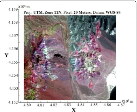
The region of this study is Cuprite mining district in Nevada, USA. The reason for this selection is the avail-ability of the field-collected samples and airborne images of AVIRIS (Figure 1). The region is a mineral research area containing different minerals such as silicas and
carbonates. The image is acquired by AVIRIS sensor on 1995 with dimensions of 350 × 400 pixels in 50 bands from 1.99 to 2.48μm. The spectral resolution of 10 nm, spatial resolution of 20 m, signal-to-noise ratio of 500, and the flight height of 20 km are the other characteris-tics of the image [9]. The image is claimed that has been corrected for the effects of atmosphere and noises using ATREM [10] and EFFORT [11], respectively. Also it is claimed that it has been corrected for the instru-mental errors [12].
3. Methodology 3.1. Data preparation
Our new technique is developed using the first two innovations of the Tetracorder, a special analysis. In what follows, the CDAF technique is introduced through its eight implementation stages. Here to prepare the images for implementing CDAF, the following few calculation steps were carried out first:
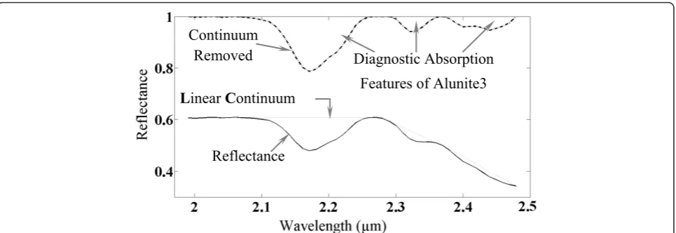
Step 1: first the CR procedure was applied to the spec-tral libraries as well as pixel spectrum. Then a linear continuum (LC) laid over the material and pixel’s reflec-tance spectrums. CR normalizes reflecreflec-tance spectra in order to allow comparison of individual absorption fea-tures from a common baseline [13]. The LC is a convex hull fitted over the top of a spectrum to connect local spectrum maxima. The first and last spectral data values are on the hull and therefore the first and last values of continuum-removed spectrum are equal to 1. The out-put curves have values between 0 and 1, in which the absorption pits and dips are enhanced. Figure 2 shows an illustration of CR and LC for Alunite3.
Step 2: a fit of every absorption features present in the pixel spectrum with those of spectral libraries can be
calculated through the standard least square method as follow [2].
Oc=a+bLc⇒
⎧ ⎪ ⎪ ⎪ ⎨ ⎪ ⎪ ⎪ ⎩
a=Oc−b
Lc n
b=
OcLc−OcLc
n
L2
c −
Lc
2
n
(1)
where aand b are coefficients of linear relationship
between CR of spectral libraryLcand CR of Observed
(pixels)Ocandnis the number of bands present in the absorption region. The reverse of this relationship was also carried out by fitting the observed valuesOc toLc
as follows:
Lc=a+bOc⇒
⎧ ⎪ ⎪ ⎪ ⎨ ⎪ ⎪ ⎪ ⎩
a=Lc−b
Oc n
b=
OcLc−OcLc
n
O2
c −
Oc
2
n (2)
Tetracorder defines fitness F between these curves
usingb andb’coefficients as shown in Equation 3 [2]:
F=bb1/2 (3)
The fitness coefficientFis assumed to be a measure of how well the spectral features match each other.
It is worthy to note that, in this study the definition of diagnostic absorption feature is slightly different from one that is used in other studies. In this study, we con-sider the whole region between two consecutive values of 1 in CR curve as a diagnostic absorption feature; where it is fully independent of its area, shape, depth, etc.
Step 3: at this stage, the weighted fitness coefficients between materials (spectral libraries) and observed
(pixels) are calculated. Note that usually every feature in the CR covers more than one absorption feature and those features with greater width contains more absorp-tion bands and consequently can better represent the relevant material [2,14]. For this, Tetracorder works on the basis of the calculated absorption area as a measure of weighting and calculates the weighting fitness for the whole spectrum of the material and pixel as:
Fw= 1 A
Na
i=1
FiAi (4)
where Ai is the area confined between CR and line
representing reflectance 1 (Figure 2) in ith absorption
region, and A represents the whole area confined
between CR and horizontal line 1,Fiis the fitness coeffi-cient (Equation 3) for theith absorption feature andFw
represents weighted fitness for all Naabsorption features present in the spectrum.
Step 4: Now the mineral corresponding to the highest weighted fitness is taken as the class of the pixel under consideration [2].
3.2. Implementation of CDAF technique
The CDAF technique is based on the first two innova-tions of Tetracorder method plus some manipulainnova-tions on the pixel and material reflectance spectrum in spec-tral libraries and their CRs. This means that the CDAF technique takes all of these curves into its calculations. The main hypothesis of this technique is based on the fact that the minerals may continuously be present in small regions such as 20 × 20 m [15], i.e., the surface distribution of a particular material does not change abruptly and this distribution could be assumed more or less similar from one region to its neighboring regions. Then, if the majority of pixels certify the presence of a
Continuum
Removed
Diagnostic Absorption
Features of Alunite3
L
inear
C
ontinuum
Reflectance
particular material, it would imply that this material could be present dominantly in the contiguous pixels too. This assumption could enable us to reduce the chance of misclassification.
In CDAF technique, two thresholds “Fitness
Thresh-old“ and“Frequency Threshold“ are used where each one of these could be determined either analytically or through some experimental procedures (if the ground truths are available). This can be done for different images of different sensors and for different conditions. In this study, these thresholds have been found to be around 80 and 70%, respectively. The procedure of implementation of this technique is presented in eight stages as follows:
Stage 1: selecting a small region (5 × 5 pixels) on the AVIRIS image. It is true that we have used 5 × 5 pixels windows in the classification procedure but this does not necessarily mean that we have lowered the spatial resolution down to 100 m. The reason for selecting this window was to expedite the calculation (reduce calcula-tion time), for example by using this window we could find 10 materials out of 481 different materials in the spectral library having more chance to be present in the pixels. These ten materials are used for second round of classification, and in this round the classification is run for each and every pixel. It is possible for a pixel to be assigned a class different from its neighbors in 5 × 5 windows in the second run.
Stage 2: applying first and second steps of Tetracorder on each pixel on the selected region using all materials present in the spectral library.
Stage 3: selecting those materials having fitness above fitness threshold (i.e, 80%) and dismiss the rest.
Stage 4: Using results of stage 3 for selection of mate-rials having frequency of more than its threshold value (here 70%).
After this stage, the number of materials suspected to be present in image is decreased dramatically and this will expedite the remaining calculations. It is worth to consider that the number of materials with highest fre-quencies determined in stage 3 is not necessarily equal to that of stage 4. So, before moving to the next stage, a criterion will be imposed in order to optimize the results. This criterion consists of an“if condition” as:
“if the ratio of the highest frequency to the total num-ber of pixels in the selected region is greater than the fre-quency threshold“
then the reflectance curves of these selected pixels would be used in the next stages (instead of their CRs), because the main hypothesis of the CDAF (i.e., the minerals may present as continuous in small regions) is fulfilled. In case the condition is not met, then CR curves of both material and pixels will be used in the next stages. Since usually this condition is always met,
then in what follows the term reflectance spectrum will be used (instead of CR).
Stage 5: at this stage, a weight will be assigned to each and every spectral band of pixels and materials. It is obvious that those bands with higher depth play more important roles in detection of the main material (the one that determines the class) and vice versa. Then, a weight proportional to the depth of each band in the CR can be given. These weights can be calculated using the following equations:
w(bdi)= BDi Nb
j=1
BDj (5)
BDi= 1−CR(pixeli) (6)
where w(bdi), BDi, and CR (i)
pixel are the calculated weights,
band depth, and CR in theith band of the pixel, respec-tively, andNbis the number of bands used in the image spectrum. Applying these weights to the pixel and mate-rial’s reflectance curves (S(i)
t andS
(i)
r ) may produce new
weighted-spectral reflectance for both pixels and materi-als (S¯(ti) and S¯(ri))
¯
Sr(i)=Sr(i)×w(bdi) (7)
¯
St(i)=St(i)×w(bdi) (8)
where r and tstand for the reference (material) and target (pixel), respectively. It is clear that these new curves are totally different with the original reflectance curves.
Stage 6: at this stage, a new weight for each material according to the area confined between curves of refer-ence material and target pixels calculated in stage 5 was defined using the following equation:
w(ai)= |
A(ri)−At|
−1
NS
j=1
|A(rj)−At|
−1 (9)
where w(i)
a is the weight for the ith material, A(ri) and
output of stage 5, the curves of stage 6 namely S˜(i)
r is produced.
˜
Sr(i)=S¯r(i)×w(ai) (10)
Figure 3 shows a sample output reflectance curve for Alunite and a pixel of the same class.
Stage 7: As shown in Figure 3b, c, applying weights in stages 5 and 6 makes the new reflectance curves of material and pixels to look similar. Naturally for those materials being principle component in the pixels (class of pixels) this similarity increases. So, a line fit between material reflectance spectrum and pixel’s spectrum does not have a width from the origin and only has a coeffi-cient of proportionality as follows:
˜
Sr=aS¯t⇒ a=
¯
STtS¯t
−1¯
STtS˜r
(11)
whereais linear relationship coefficient and S¯Tt is the transpose of S¯t (Figure 3c).
Stage 8: At this stage, using coefficient of proportion-ality (found in previous stage) “a“, the material new spectrum S˜r will be estimated from pixel new spectrum
¯
St (Figure 3c). Then, the root mean square error
(RMSE) between pixel and material new spectrum can be calculated.
˜
Sr=aS¯t⇒ RMSEr=
Nb
i=1
˜
S(ri)− ˜S(ri)
2
Nb−1
(12)
Now the material that minimizes these RMSEs is taken to be the class of that pixel. Here,Nbis the num-ber of bands being used.
4. Results and analysis
To test the suggested technique and to analyze the results, the following data have been used:
a AVIRIS images explained in Section 2.
b Field collected data for five classes of materials (Table 1).
c Reflectance curves for 481 different materials collected by USGS available in ENVI software. The spectral library of the minerals can also be found in the USGS website http://speclab.cr.usgs.gov/spectral-lib.html.
4.1. Technique evaluation
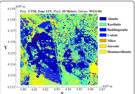
Here CDAF technique has been programmed in MATLAB and executed on the AVIRIS image and the results are shown in Table 2. The overall accuracy achieved in this technique was 96.9% (126 out of 130). The map produced by this technique is shown in Figure 4.
5. Discussion
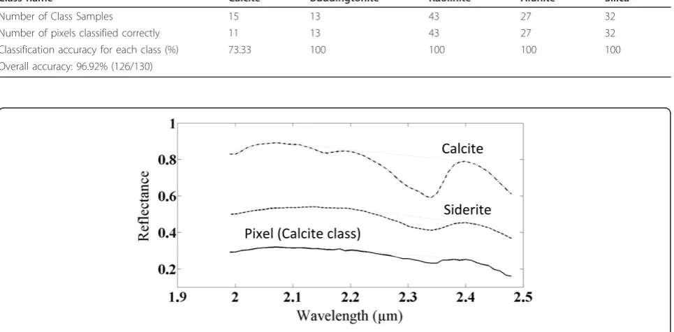
Results of the CDAF technique shown in Table 2 prove its ability in classification of Alunite, Buddingtonite, Kaolinite, and silica perfectly, meaning that the imposed conditions and performed calculations in CDAF techni-que have proven its robustness. As shown in Table 2, the classification precision in the class of calcite is lower compared to the other classes although the results are still acceptable. This situation comes from the fact that there might exist some material in the spectral library having reflectance more similar to the reflectance of the pixel rather to that of calcite (Figure 5). On the other hand, regarding discussion in Section 2, we only used the spectral region confined between 2 and 2.5μm. This
(b)
(c)
(a)
Alunite
Pixel
renders discrimination of the group of materials (in the same family) having similar absorption signature very difficult. For instance, calcite and siderite both are from carbonate family and their reflectance curves in 2 to 2.5
μm have similar absorption region (Figure 5) and conse-quently the chance of their discrimination with the spectral-based techniques are very low. Also as can be seen from Figure 5, the reflectance curve of siderite (FeCO3) and one of the calcite (CaCO3) class pixels are
very similar to each other while this similarity for the pair of calcite-pixel is much lower. Then to discriminate calcite from siderite, we need more spectral information (e.g., 0.4-2.5 mm) whereas this would be a restriction with the current data.
The robustness of the CDAF is more profound in some special circumstances. One of these cases is the class of silica. There are varieties of silicas different in names but more or less with high similarity in the absorption features in their reflectance curves. Adding
to this, the soils reflectance with special characteristics due to their physical and chemical particulars while their main constituents are minerals, organic materials, air, and water [10,16]. These pixels were classified with 100% accuracy using CDAF technique. The reason for this is the analytical procedure introduced in the techni-que. Table 2 shows that by removing calcite from the list of classes, the classification precision raises from 96.92 to 100% where this itself is a great step in the classification of hyperspectral images [8].
Finally, it is worth noting that we have run our tech-nique based on the field collected data by other people in the Cuperite field campaign where we ourselves did not play any role in that. As can be seen from Table 2, the CDAF technique could detect four of the classes with 100% accuracy and only has weakness in detec-tion of calcite class (73.33%). However, it is possible that the field work done by the other people on the class of calcite was not accurate enough and had some misinterpretations involved. For example, it is possible in some region, the siderite abundance was more than calcite but the people collected the samples gave the calcite class. On the other hand, the accuracy of 100% does not necessarily means that there are no other material present in the pixel but it could be concluded that the combination of abundance and absorption features of on material has influenced the pixel reflec-tance to render the shape to look like a particular class.
Table 1 Characteristics of 5 materials in 130 samples used in method testing and analysis
Class Material number in the list of ENVI spectral library
Number of labeled samples
Alunite 23-28 27
Kaolinite 233-240 43
Buddingtonite 67 and 68 13
Calcite 72-74 15
Silica 88, 91, 380-383, 345-346 32
Table 2 Results of classification and overall accuracy of CDAF method
Class name Calcite Buddingtonite Kaolinite Alunite Silica
Number of Class Samples 15 13 43 27 32
Number of pixels classified correctly 11 13 43 27 32
Classification accuracy for each class (%) 73.33 100 100 100 100
Overall accuracy: 96.92% (126/130)
Pixel (Calcite class)
Calcite
Siderite
6. Conclusion
In this study, based on the first two stages of Tetracor-der method, a new technique called CDAF is developed. This technique enables one to classify the minerals with high precision. The technique is based on the derivation of information from the image reflectance spectrum. This can be done through extraction of spectral absorp-tion features of any minerals from their corresponding laboratory-measured reflectance spectra, and comparing it with those extracted from the image. The results of evaluation show acceptable and reliable performance of the suggested technique. In this study, along with the first two innovations of Tetracorder method, based on absorption depth and absorption areas in the CR of reflectance curves, some weighting coefficients are cal-culated. These weighting coefficients help classification of pixels through their spectral similarities to a particu-lar substance. The significance of CDAF technique is that in this technique besides using absorption features in the material and pixel in the respective CR of reflec-tance curves, the reflecreflec-tance curves themselves are being used as well. Considering the results of classification, it can be seen that CDAF can perform well in all classes and can be applied to the region with the high variety of minerals distributing in a continuous manner. On the other hand, the results shown in Table 2 prove that this technique has been able to perform 100% accuracy in classification for most of the cases. So, the CDAF technique is recommended as a good substitution for unsupervised classification techniques in hyperspectral images.
Competing interests
The authors declare that they have no competing interests.
Received: 11 February 2011 Accepted: 14 November 2011 Published: 14 November 2011
References
1. BC Kuo, DA Landgrebe, Improved statistics estimation and feature extraction for hyperspectral data classification, PhD thesis, School of Electrical & Computer Engineering Technical Report. Purdue University, USA, (2001)
2. RN Clark, GA Swayze, KE Livo, RF Kokaly, SJ Sutley, B Dalton, RR McDougal, CA Gent, Imaging spectroscopy: earth and planetary remote sensing with the USGS Tetracorder and expert systems. J Geophys Res.108, 1–44 (2003), http://speclab.cr.usgs.gov/PAPERS/tetracorder
3. GR Hunt, JW Salisbury, Visible and near-infrared spectra of minerals and rocks. I. Silicate minerals. Mod Geol.1, 283–300 (1970)
4. RN Clark, TVV King, M Klejwa, GA Swayze, N Vergo, High spectral resolution reflectance spectroscopy of minerals. J Geophys Res.95, 12653–12680 (1990). doi:10.1029/JB095iB08p12653
5. RN Clark, inSpectroscopy of Rocks and Minerals, and Principles of Spectroscopy, Manual of Remote Sensing, Remote Sensing for the Earth Sciences, vol. 3, ed. by Rencz AN (Wiley, New York, 1999), pp. 3–58 6. MR Mobasheri, Y Rezaie, MJ Valadan-zouje, A method in extracting
vegetation quality parameters using hyperion images, with application to precision farming. World Appl Sci.2, 476–483 (2007)
7. RN Clark, GA Swayze, R Wise, KE Livo, TM Hoefen, RF Kokaly, SJ Sutley, 2000-2007, USGS Digital Spectral Library, http://speclab.cr.usgs.gov/spectral-lib.html
8. RN Clark, TL Roush, Reflectance spectroscopy: quantitative analysis techniques for remote sensing applications. J Geophys Res.89, 6329–6340 (1984). doi:10.1029/JB089iB07p06329
9. FA Kruse, JW Boardman, JF Huntington, Comparison between AVIRIS and hyperion for hyperspectral mineral mapping. IEEE Trans Geosci Remote Sens.41, 1388–1400 (2003). doi:10.1109/TGRS.2003.812908
10. BC Gao, AFH Goetz, Column atmospheric water vapor and vegetation liquid water retrievals from airborne imaging spectrometer data. J Geophys Res.
95, 3549–3564 (1990). doi:10.1029/JD095iD04p03549
11. JW Boardman, Post-ATREM polishing of AVIRIS apparent reflectance data using EFFORT: a lesson in accuracy versus precision, inProceedings of the 8th JPL Airborne Earth Science Workshop, Jet Propulsion Laboratory Publication 99-17, p. 53 (1998)
12. RN Clark, GA Swayze, KE Livo, RF Kokaly, TVV King, JB Dalton, JS Vance, BW Rockwell, T Hoefen, RR McDougal, Surface reflectance calibration of terrestrial imaging spectroscopy data: a tutorial using AVIRIS, inProceedings of the 10th Airborne Earth Science Workshop, JPL Publication 02-1, (2002) 13. RF Kokaly, Investigating a physical basis for spectroscopic estimates of leaf
nitrogen concentration. Remote Sens Environ.75, 153–161 (2001). doi:10.1016/S0034-4257(00)00163-2
14. GA Swayze, RN Clark, AFH Goetz, TG Chrien, NS Gorelick, Effects of spectrometer band pass, sampling, and signal-to-noise ratio on spectral identification using the Tetracorder algorithm. J Geophys Res (Planets).
108(E9), 5105 (2003)
15. J Zhang, B Rivard, DM Rogge, The successive projection algorithm (SPA), an algorithm with a spatial constraint for the automatic search of
endmembers in hyperspectral data. Sensors.8, 1321–1342 (2008). doi:10.3390/s8021321
16. FD Van Der Meer, SM Dejong,Imaging Spectrometry: Basic Principles and Prospective Applications(Delft University of Technology, Kluwer Academic Publishers, 2002), pp. 11–12. 47, 71–80
doi:10.1186/1687-6180-2011-102
Cite this article as:Mobasheri and Ghamary-Asl:Classification by diagnosing all absorption features (CDAF) for the most abundant minerals in airborne hyperspectral images.EURASIP Journal on Advances in Signal Processing20112011:102.