Volume 2009, Article ID 416395,12pages doi:10.1155/2009/416395
Research Article
Self-Localization and Stream Field Based Partially
Observable Moving Object Tracking
Kuo-Shih Tseng
1and Angela Chih-Wei Tang
21Intelligent Robotics Technology Division, Robotics Control Technology Department, Mechanical and System Laboratories,
Industrial Technology Research Institute, Jiansing Road 312, Taiping, Taichung 41166, Taiwan
2Visual Communications Lab, Department of Communication Engineering, National Central University,
Jhongli, Taoyuan 32054, Taiwan
Correspondence should be addressed to Kuo-Shih Tseng,[email protected] Received 30 July 2008; Revised 8 December 2008; Accepted 12 April 2009 Recommended by Fredrik Gustafsson
Self-localization and object tracking are key technologies for human-robot interactions. Most previous tracking algorithms focus on how to correctly estimate the position, velocity, and acceleration of a moving object based on the prior state and sensor information. What has been rarely studied so far is how a robot can successfully track the partially observable moving object with laser range finders if there is no preanalysis of object trajectories. In this case, traditional tracking algorithms may lead to the divergent estimation. Therefore, this paper presents a novel laser range finder based partially observable moving object tracking and self-localization algorithm for interactive robot applications. Dissimilar to the previous work, we adopt a stream field-based motion model and combine it with the Rao-Blackwellised particle filter (RBPF) to predict the object goal directly. This algorithm can keep predicting the object position by inferring the interactive force between the object goal and environmental features when the moving object is unobservable. Our experimental results show that the robot with the proposed algorithm can localize itself and track the frequently occluded object. Compared with the traditional Kalman filter and particle filter-based algorithms, the proposed one significantly improves the tracking accuracy.
Copyright © 2009 K.-S. Tseng and A. C.-W. Tang. This is an open access article distributed under the Creative Commons Attribution License, which permits unrestricted use, distribution, and reproduction in any medium, provided the original work is properly cited.
1. Introduction
Navigation in a static environment is essential to mobile robots. The related research topics consist of self-localization, mapping, obstacle avoidance, and path planning [1]. In a dynamic environment, it becomes interactive navigation including leading, following, intercepting, and people avoid-ance [2]. The major concern of following is how to track and to follow moving objects without getting lost. In this scenario, the robot should be capable of tracking, following, self-localization, and obstacle avoidance in a previously mapped environment. Following and obstacle avoidance are the problems of decision making while object tracking and robot localization are the problems of perception. A good perception system improves the accuracy of decision making. Robots with the ability of object tracking can accomplish complex navigation tasks easier. In this paper, we focus
on object tracking and robot localization for interactive navigation applications.
Robot Object
(a)
Robot Object
Obstacle
(b)
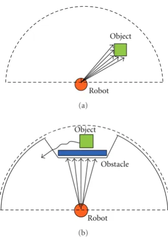
Figure 1: A fully observable object and a partially observable object. The dash line is the scan range of laser, the solid line is the observable range of laser for unobservable case, and the arrow is scanned points of laser. (a) Observable moving object tracking. (b) Unobservable moving object tracking.
can be tracked with higher accuracy although the price is high computational complexity [5,6]. SLAMMOT uses scan matching and EKF with a laser range finder to simultaneously estimate the robot position, map, and states of moving objects [7]. Furthermore, the local grid-based SLAMMOT adopts incremental scan matching to reduce the computational complexity and improve the reliability in dynamic environments [8]. SLAMIDE can also estimate the robot position, map, and states of moving objects as SLAMMOT. However, SLAMIDE does not need to categorize objects into dynamic and static ones with reversible data association [9]. The conditional particle filter can estimate the people motion conditioned on the robot position with a previously mapped environment [2]. To achieve the better prediction precision of the object motion, most tracking algorithms employ the interacting multiple model (IMM) as the motion model of the Kalman filter or particle filter [10]. Without the corrections based on the sensor data, they predict the inflated Gaussian distribution or dispersed particles of the object states. Such algorithms are effective only if the object is observable (Figure 1(a)) [2, 4], and they fail in the unobservable case as shown
in Figure 1(b). In this paper, the tracking problem where
a robot can still observe the environment except hidden objects is called partially observable moving object tracking (POMOT).
In [11], a map-based tracking algorithm using the Rao-Blackwellised particle filter (RBPF) concurrently estimates the robot position and ball motion. It models the physical interaction between the wall and the ball even if the ball
is unobservable (Figure 1(b)). The authors also propose a tracking algorithm conditioned on Monte Carlo localization and this algorithm can track passive objects successfully. This algorithm considers two kinds of samples where one is for object position and the other is for object velocity [12]. For visual tracking, a Bayesian network-based scene model reasoning the object state can be utilized when the target is occluded [13, 14]. The information of the local color, texture, and spatial features relative to the centers of objects assists the online sampling and position estimation [15]. The occlusion problem can be also solved with the aid of depth maps [16]. However, such image processing techniques cannot be applied to the laser range finder data since there is neither 2D foreground information or the partially unoccluded object information available. Currently, most laser-based tracking algorithms will fail if the object is unobservable.
Therefore, in this paper, we propose a novel laser based self-localization and partially observable moving object tracking (POMOT) algorithm. Since the object motion is significantly influenced by the environments and object goal, we adopt a stream field-based motion model proposed in [17] and combine it with the Rao-Blackwellised particle filter (RBPF) to predict the object goal and then compute the object position with known environmental informa-tion. Since POMOT is a nonlinear and multihypotheses problem, we adopt the RBPF as our estimator. With the stream field, we can model the interactions among the goal position, environmental features, and object position. In the traditional tracking algorithms, objects are considered to move actively with the velocity and acceleration generated by themselves. But from the viewpoint of the stream field, object motion is deemed to be passive due to the attraction and rejection forces between the object goal and environment. The proposed algorithm can still keep predicting the object position based on the known stream field even if the object is unobservable. Moreover, a robot can localize itself and track moving objects according to the virtual stream field.
The rest of the paper is organized as follows.Section 2
describes the adopted motion model using the stream field for object tracking. In Section 3, our proposed tracking algorithm which combines the stream field and RBPF is presented. Also, we propose our self-localization and object tracking algorithm. Experimental results are given in
Section 4, and finallySection 5concludes this paper.
2. The Stream Field-Based Motion
Model for POMOT
model for the proposed tracking algorithm. The advantages are stated as follows. First, the stream field constructs an active field where the object is moved inactively due to the attraction and rejection forces in the stream field. Based on this, we can predict the object position according to the known stream field even if the object is unobservable. Secondly, the stream field-based motion model can be easily integrated with any object tracking algorithm. Therefore, a robot can estimate the object position and follow the object based on the same stream field without another path planning algorithm.
InSection 2.1, we will introduce how to carry out motion
planning using the stream field.
2.1. Motion Planning Using Stream Field. The complex potential is often adopted to solve the problems of fluid mechanics and electromagnetism [22]. It is one of the representations of the stream functions. For an irrational and incompressible flow, there exists a complex potential which consists of the potential functionφ(x,y) and stream function
ψ(x,y), where (x,y) is the 2D coordinate. The complex potential is defined by
w=φ+iψ=f(z), z=x+iy,
∂φ ∂x =
∂ψ ∂y,
∂ψ ∂x = −
∂φ ∂y.
(1)
Then, the velocitiesvx along thex-axis andvy along the y
-axis can be derived by the stream function
vx= ∂ψ
x,y
∂y , vy= −
∂ψx,y
∂x . (2)
Simple flows include uniform flow, source, sink, and free vortex. The complex potential can be formed by these simple flows with various combinations. In this paper, we use a sink and a doublet flows which combines a sink and a source flow. The stream functions of the sink flow, source flow, and the doublet flow are
ψsink
x,y=Ctan−1
y x
,
ψsourcex,y= −Ctan−1 y
x
,
ψdoubletx,y= −Ctan−1
y x2+y2
,
(3)
whereCis a constant in proportion to the flow velocity. There are four major methods to define various complex potentials for real environments: simple flow, use of specific theorems, conformal mapping, and a panel method [23]. We adopt specific theorems to construct the stream function for motion planning. As shown inFigure 2, we assume the
S G
(a) (b)
Figure2:Gis the goal,Sis the starting point, and the solid circle is an obstacle. (a) Obstacle avoidance. (b) Stream field.
robot will move toward the goal from the starting point. The obstacle is located between the goal and the starting point. Thus, we can model the environment as a stream field where the goal is a sink flow and the obstacle is a doublet flow.
According to the circle theorem, we get the stream field which consists of a sink flowψsink(x,y) and a doublet flow
ψdoublet(x,y) by [20], and
ψx,y
=ψsink
x,y+ψdoubletx,y
= −Ctan−1
y−ys
x−xs
+Ctan−1 ⎛ ⎝a2
y−yd
/(x−xd)2+
y−yd
2
+yd−ys
a2(x−x
d)/
(x−xd)2+
y−yd
2
+ (xd−xs)
⎞ ⎠,
(4)
where (xs,ys) is the center of sink, (xd,yd) is the center of
doublet,a is the radius of doublet, andC is the constant proportion to the flow velocity. More details of the stream field derived by the circle theorem can be found in [20]. Finally, the stream functions can be computed when the robot position, object goal, and obstacle position are known. The desired robot velocities is computed by (2), and the headingθdis
θd=tan−1
−∂ψx,y/∂x
∂ψx,y/∂y
. (5)
With these, robots are capable of realizing real-time motion planning. InSection 2.2, we will describe the stream field-based motion model in the proposed tracking algorithm.
Interactive multiple-model (IMM), constant velocity and acceleration model are often adopted in the motion models [24]. However, in the unobservable case, the motion model of the prior transition probability of the Kalman filter or particle filter predicts the inflated Gaussian distribution or dispersed particles of object states without the corrections of sensor information. One possible solution is the off-line learning-based tracking algorithm where the destination is learned, the candidates for the goal can be found through learning the trajectories. Then the tracking accuracy is improved by referencing the possible object paths generated based on the destination information [25]. In [26], another learning based people tracking algorithm is realized with the Hidden Markov Model (HMM) where the expectation maxi-mization (EM) is applied to laser range finder (LRF) data for learning. In this paper, we adopt a stream field-based motion model proposed in [17]. With this, we can on-line predict the motion path according to the known map features and the virtual goal. The advantage of our stream field-based motion model is that it can track the unobservable object position successfully. In object tracking, the object position at timet
is
xt= f(xt−1,vt−1), (6)
wherevt−1is the object motion at timet−1.
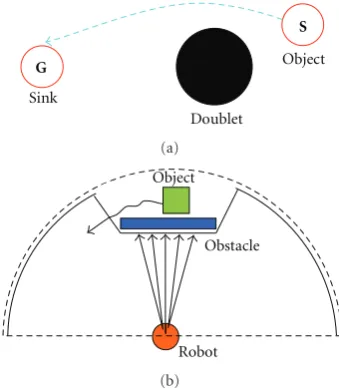
As shown in Figure 3(b), the robot cannot track the moving object efficiently when the object is unobservable. Thus, we assume that objects will avoid the known obstacle and move toward the virtual goal as in the stream field
(Figure 3(a)). By (4), the stream field is generated based
on the object goal, object state, and environment. A virtual sink and a doublet resulted from a known environment construct a stream field, and the object motion is predicted by
Vt−1=
vo,t−1 vo,t−1
= ⎡ ⎢ ⎢ ⎢ ⎢ ⎣
∂ψsink
xo,t−1,yo,t−1
+ψdoubletxo,t−1,yo,t−1
∂yo,t−1
−∂
ψsink
xo,t−1,yo,t−1
+ψdoubletxo,t−1,yo,t−1
∂xo,t−1
⎤ ⎥ ⎥ ⎥ ⎥ ⎦,
(7)
where (xo,t−1,yo,t−1) is the object position at timet−1.
Our stream field-based tracking algorithm estimates the object position after estimating the virtual goal position and flow intensity. Then the object motion is predicted based on the virtual goal and known obstacle information where the object velocity and acceleration are not estimated directly. How to estimate the virtual goal position of a partially observable moving object is a multihypotheses problem. For this, we adopt the particle filter to estimateNpossible goal positions. In the next section, we will present our object tracking algorithm using the stream field-based motion model in the Rao-Blackwellised particle filter.
S
G
Doublet Sink
Object
(a)
Robot Object
Obstacle
(b)
Figure3: Illustrations of the stream field-based motion model and real environment. (a) Stream field-based motion model. (b) A real environment.
3. The Proposed Localization and
Partially Observable Moving Object
Trakcing Algorithm
3.1. POMOT Using the Stream Field-Based Motion Model and RBPF. To achieve accurate motion prediction, we incorporate the stream field-based motion model with our tracking algorithm. The proposed graphical model is shown in Figure 4(b), and it is quite different from the traditional tracking algorithms (Figure 4(a)). InFigure 4(a), the prediction stage of tracking will diverge if there is no effective measurement of object information. However, our RBPF based algorithm using the stream field-based motion model will achieve effective prediction by a virtual sink flow and doublets generated from obstacles even without effective measurements (Figure 4(b)). In the POMOT case, the RBPF based object tracking will perform well due to its multihypotheses if the object is sheltered from its environment.
The particle filter is widely adopted as the kernel of objects tracking. It can predict and correct states with arbi-trary nonlinear probability distribution and n-hypotheses. However, the major disadvantages are its assumptions. First, it is hard to predict the accurate probability distribution of object motion by the n-hypotheses. Secondly, the computa-tional complexity of the particle set grows exponentially with the number of tracked variables.
The particle filter is stated as follows. We assume that
Okis the object state at timek, andzk is the measurement
at time k. The particle filter estimates the state of moving objects through predictions and corrections. The prediction stage is to sample the state probability distribution by a set of particles
Oik∼q
Oik|Oik−1,zk
Object location
Object detection
MO
T
Zt−1 Zt Zt+1
Ot−1 Ot Ot+1
(a)
Object detection Object location Doublet
Sink
POMO
T
Zo
t−1 Zto Zt+1o
Ot−1 Ot Ot+1
Gt−1 Gt Gt+1
Dt−1 Dt Dt+1
(b)
Robot location
Robot control
Landmark detection
Map (doublet)
Object detection Object location Sink
POMO
T
Localiza
r
tio
n
Zto−1 Zot Zt+1o
Ot−1 Ot Ot+1
Gt−1 Gt Gt+1
m ZLt−1
ut
ut−1
ZL t
ut+1
Zt+1L
rt−1 rt rt+1
(c)
Figure4: Dynamic Bayesian Networks (DBNs) of (a) traditional tracking, (b) stream field-based tracking, and (c) localization and tracking.
The correction stage computes the weightingwki of the ith
particle at timekby
wik∝wik−1
pzk|Oik
pOik|Oik−1
qOik|Oik−1,zk
. (9)
When the moving object is sheltered by the environments or moving obstacles, the measurementzt is invalid for the
correction stage. In the POMOT case, an accurate proposal distribution is helpful to keep predicting without corrections. Our stream field-based motion model aims at predicting the object position and object goal. Nevertheless, the com-putational load of the particle filter to sample and compute
weightings of stream sample setSkis pretty heavy where
Sk=
sik,wik|1≤i≤N
,
Sik=Oi
k,Gik,D
=Ox,k,Oy,k,ΣO,k
i
,Gφ,k,Uk
i
,D
,
(10)
where Oi
k is the object state of the ith particle at time k
including the mean (Ox,k,Oy,k) and covariance ΣO,k. The
object goalGikincludes the directionGφ,kand intensityUk.D
is the doublet position generated by the previously mapped features.
The major problems of the implementation of the stream field-based tracking algorithm are stated as follows. First, it is a multihypotheses and nonlinear problem. Secondly, it needs a precise probability distribution model to predict the POMOT case. Third, the number of scalars of the state vectorSkis large so that the computational complexity of the
particle filter is high. The first problem used to be solved by the particle filter while the third one used to be solved by the Kalman filter. However, it is improper to adopt either Kalman filter or particle filter for the second problem. Thus, we combine the stream field-based motion model with the Rao-Blackwellised particle filter in the tracking algorithm. The RBPF is capable of solving the n-hypotheses problem and it approximates the probability distribution function more precisely [27–29]. In our RBPF based tracking algorithm, the particle filter estimates the goal states Gik and the Kalman
filter estimates the object state Oik. A stream sample set
includes the object stateOi
k, goal stateGit, and doublet D.
In a known feature map, doublets are fixed. The stream field-based tracking distribution is decomposed from the factorization of the probability as follows:
bel(Sk)=P(S1:k|z1:k)
=POi
k,Gik,O1:ik−1,Gi1:k−1,D|z1:k
=PGi
k|Oik,Oi1:k−1,Gi1:k−1,D,z1:k
×POi
k|Oi1:k−1,Gi1:k−1,D,z1:k
×POi
1:k−1,Gi1:k−1,D|z1:k
(11)
DBN
= PGik|Oik,Gik−1
×POik|Oi1:k−1,Gi1:k−1,D,z1:k
×POi1:k−1,Gi1:k−1,D|z1:k−1
(12)
markov
= P(Gik|Oik,Gki−1)
goal set sampling
P(Oki |Oki−1,D,Gik−1,zk)
object set distribution
×P(Oi
k−1,Gik−1,D|zk−1)
bel(Sk−1)
.
(13)
Here, (12) is derived based on the independencies in the graphical model inFigure 4(b), and (13) is due to the Markov property. The goal probability distributionP(Gik |
Oik,Gik−1) in (13) can be randomly sampled based on the
Object
Obstacle Sink
(a)
Object
Obstacle Sink
Stream line
(b)
Object
Obstacle Sink
Stream line
Predicted object
(c)
Object
Obstacle
Measured object
Correct object
(d)
Object
Obstacle
Measured object 0.6 0.2
0.2
(e)
Object
Obstacle
Measured object Sink
0.6 0.2 0.2 (f)
Figure5: Steps of stream field-based tracking algorithm. Prediction steps are (a), (b), and (c). Correction steps are (d), (e), and (f). The numbers within dash squares are the weighting of every predicted object position. (a) Sample of five sink flows. (b) Compute five velocities using stream function. (c) Compute five hypotheses of object position by estimated velocity. (d) Update measurement and Kalman filter. (e) Compute the normalized. (f) Resampling. (Green squares and blue squares are predicted and corrected particles, resp. The number in blue squares is weighting value of the particle.)
We factorize the stream field-based tracking distribution into the goal set distribution, object set distribution, and stream set distribution at time k−1.Based on the stream set distribution at time k−1, we assume that the distance between the object and the goal is fixed at 200 cm so that we only randomly sample the sink flow directionGφ,kand sink
flow intensityUk for efficiency. After samplingN kinds of
goal positions (Figure 5(b)), the object set distribution can be derived based on Bayes theorem as follows:
POi
k|Oi1:k−1,Gi1:k−1,D,z1:k
=P
Oi
k,Oi1:k−1,Gi1:k−1,D,z1:k−1|zk
POi
1:k−1,Gi1:k−1,D,z1:k−1|zk
Bayes
= P
zk|Oki,Oi1:k−1,Gi1:k−1,D,z1:k−1
Q
POi
1:k−1,Gi1:k−1,D,z1:k−1|zk
P(zk)
DBN= P
zk|Oik
POi
k,Oi1:k−1,G1:ik−1,D,z1:k−1
POi
1:k−1,Gi1:k−1,D,z1:k−1,zk
=P
zk|Oik
POi
k|O1:ik−1,G1:ik−1,D,z1:k−1
P(zk|z1:k−1)
=η P(zk|Oik)
object Correction
P(Oik|Oi1:k−1,Gi1:k−1,D,z1:k−1)
object Prediction
, (14)
whereQdenotesP(Oik,Oi1:k−1,Gi1:k−1,D,z1:k−1).
In Figure 5(c), Oik is computed by the stream
field-based motion model P(Oki | Oik−1,Gik−1,D) in (4) and
(14), and it is updated by the Kalman filter (Figure 5(d)). Then we compute the weightings in Figure 5(e) according to the Gaussian distribution. Finally, the stream sample set is resampled according the weightings (Figure 5(f)). This algorithm can predict the particle state Ok
accu-rately when the object is unobservable. The tracking and localization algorithm will be presented in the next section.
3.2. Localization and POMOT Algorithm. Effective predic-tion of the sheltered object mopredic-tion relies on robust local-ization and tracking. In fact, it is difficult to predict the object motion if the object has been sheltered for a long time. To achieve effective prediction, a robot has to move toward the sheltered zone and get more information related to the target object (Figure 6). In [30], the integrated method predicts the object state by the particle filter, and the robots move toward the object based on the potential field. In this section, we further incorporate the POMOT proposed in
Section 3.1 with the localization algorithm for the robust
The localization and stream sample set is
Xk=
rk,Sik|1≤i≤N
,
Xk=
rk,Sik
=rx,k,ry,k,rθ,k,Σr,k
,Ox,k,Oy,k,ΣO,k
i
,Gφ,k,Uk
i
,D
.
(15)
The localization and stream-based tracking distribution is decomposed from the factorization of the probability distribution as follows:
bel(Xk)=P(X1:k|u1:k,z1:k)
=POi
k,O1:ik−1,Gik,Gi1:k−1,rk,r1:k−1D|u1:k,z1:k
=PGi
k|Oik,O1:ik−1,Gi1:k−1,rk,r1:k−1,D,u1:k,z1:k
×POki |O1:ik−1,Gi1:k−1,rk,r1:k−1,D,u1:k,z1:k
×Prk|O1:ik−1,Gi1:k−1,r1:k−1,D,u1:k,z1:k
×PO1:ik−1,Gi1:k−1,r1:k−1,D|u1:k,z1:k
DBN
= P(Gik|Oki,Gki−1)
goal set distribution
×P(Oki |O1:ik−1,G1:ik−1,rk,D,u1:k,z1:k)
object set distribution
×P(rk|r1:k−1,D,u1:k,z1:k)
robot distribution
×P(Oi
1:k−1,Gi1:k−1,r1:k−1,D|u1:k,z1:k)
bel(Xk−1)
.
(16)
Our localization and RBPF-based tracking algorithm is fac-torized into the goal set distribution, object set distribution, robot distribution, and the last state set distribution at time
k −1 in (16). Object tracking is similar to (12) but it is conditioned on the robot position where the uncertainty of the robot localization is taken into account,
POik|O1:ik−1,Gi1:k−1,r1:k,r1:k−1,D,u1:k,z1:k
=ηP(zkO|Oik,rk)
object Correction
P(Oik|Oi1:k−1,Gi1:k−1,r1:k,D,u1:k,z1:k−1)
object Prediction
.
(17)
Robot localization is independent of the object state and object goal so that we can simplify it to be an EKF localization problem as follows:
P(rk|r1:k−1,D,u1:k,z1:k)
=ηP(zLk|rk,D)
Robot Correction
P(rk|r1:k−1,u1:k)
Robot Prediction
. (18)
More details of EKF localization derived based on the Bayes filter can be found in [31].
Our localization and RBPF-based tracking algorithm is summarized in Algorithm 1 and it is stated as follows.
Robot Object Obstacle Sink
Stream line
(a)
Sink
Robot Object Obstacle
(b)
Figure6: Localization and stream field-based tracking in (a) fully observable case and (b) POMOT.
The inputs are the stream sample set Sk−1 at time k −
1, measurement zk, and control information uk (line 1).
The stream sample set Sk−1 includes the sample set of
object goal Gk−1 and the sample set of object position Ok−1. The algorithm predicts the robot position using the
motion model of EKF localization (lines 3 and 4). All laser measurements are represented as line features using the least square algorithm. If the feature is associated with the known landmarks (line 7), the robot position will be corrected using EKF (rbpflines 8–10). Otherwise, the feature is tracked by RBPF (lines 14–21). The covariance of motion noise at time
k is Rk, the covariance of sensor noise at time k is Qk,
the predicted and corrected means of robot state at timek
areμk andμk, respectively, and the predicted and corrected
covariances of the robot state at time k are Σk and Σk,
respectively. Goal statesGik are sampled first (line 15), and
theNpossible object statesOki are predicted according to the
stream field-based motion model in (4) (line 16). If theith particle is associated with the moving object, the RBPF will update the moving object positionOi
k, and it is described
as follows. First, the algorithm computes the weighting of theith particlewi
k (line 20). Then, particles are resampled
according to their weightings (line 22). In the observable case, the stream sample setSi
k including the object sample
set Oi
k and the goal sample set Gik will converge. In the
unobservable case, it will keep predicting the object sample setOi
kbased on the previous stream fieldSik−1.
4. Experimental Results
(1) Inputs:
Sk−1= {G(i)k−1,O (i)
k−1,D |i=1,. . .,N}posterior at timek−1
uk−1 control mesurement
zk observation
(2)Sk:=ϕ //Initialize
(3)μk=g(uk,μk−1) //Predict mean of robot postion (4)Σk=GkΣk−1GTk+Rk //Predict covairance of robot postion (5) form:=1,. . .,Mdo //EKF Localization update (6) forc:=1,. . .,Cdo
(7) ifdL
m< dLthdo //ifdm< dth,ziis landmarkm
(8) Kc
k=ΣkHkcT(HkcΣkHkcT+Qk)−1 (9) μk=μk+Kkc(zck−hck(μk)) (10) Σk=(I−KkHkc)Σk (11) else do
(12) zo
c=zc //zc is a dynamic feature (13)w(i):=0
(14) fori:=1,. . .,N do //RBPF Tracking (15) Gi
k∼p(Gik|Oki,Gik−1) //virtual goal smapling (16) Oi
k∼p(Oik|Oi1:k−1,Gi1:k−1,r1:k,D,u1:k,z1:k−1) //(4) and (6) (17) for j:=1,. . .,J do //data association
(18) ifdo
m< dothdo
(19) Oi
k:=kalman update (Oik) //update object
(20) wi
k:=p(zk,jo |Oti) //compute weighting (21) Sk:=Sk∪ {G(i)k−1,O
(i)
k−1} //insertStinto sample set (22) Discard smaples inStbased on weightingwti(resampling) (23) returnSt, μt, Σt
Algorithm1: Localization and stream-based tracking algorithm.
Figure7: The mobile platform Ubot.
the computing platform to verify our algorithm (Figure 7). UBOT is developed by ITRI/MSRL in Taiwan, and it is equipped with one SICK laser. We use PhaseSpace to generate the precise ground truth of the trajectories of people and robot [32]. PhaseSpace is an optical motion capture system, and it estimates the LED markers’ position, velocity, and acceleration with eight cameras. The measurement accuracy depends on the calibration where the calibration accuracy is 1.4510 mm. We use four LED markers where two for the robot and the others for the people legs for the position measurement, respectively.
The accuracy of people tracking will be improved if the laser is mounted higher. This is due to the fact that torso tracking is easier than leg tracking since the torso is
more rigid than legs. However, the laser is usually mounted lower to measure the environmental landmarks in the localization applications and to sense the obstacles at the same time. Based on the issue of simultaneous verification of localization and object tracking algorithm, we mount the laser at the low height for self-localization and people tracking. Our system and PhaseSpace runs at 4 Hz and 120 Hz, respectively. The ground truth is the average of thirty data at continuous time instants from PhaseSpace. The average of position of two legs is deemed as the people’s position. Our tests show that the probability that the system cannot recognize the LED marker is less than 1%. In such case, we generate the unrecognized data by interpolation.
In the following, we design three experiments to verify performance of the proposed algorithm. First, we compare the tracking performance of the Kalman filter, particle filter, and RBPF when the object is observable. Next, we compare the tracking performance of the Kalman filter, particle filter, and RBPF for the partially observable object. Also, the experiment of localization with EKF and odometer data is conducted. Finally, the performance of PF using the stream based motion model and RBPF using the stream field-based motion model are compared.
Robot
People Goal
(a) (b)
Figure 8: Object tracking experiment. (a) People trajectory. (b) Experimental environment.
Table1: Comparisons of errors in cm of KF, PF, and RBPF using stream field-based tracking algorithms.
KF PF RBPF-SF
Total error mean 11.3 10.7 10.2
Total error std. 6.1 5.7 5.2
Table 2: Comparisons of tracking errors in cm of EKF and odometer.
Odometer EKF
Total mean 8.1 5.7
Total Std. 4.3 3.9
the black ellipse line once. Kalman filter (KF) adopts the constant velocity model, SIR particle filter (SIR PF) is with 1000 particles, and RBPF using stream field-based motion model (RBPF-SF) with 1000 particles. Table 1 and
Figure 9 summarize the error data of five experiments.
The total average tracking errors of KF, PF, and RBPF-SF are 11.3 cm, 10.7 cm, and 10.2 cm, respectively. The total standard deviations of tracking errors of KF, PF, and RBPF-SF are 6.1 cm, 5.7 cm, and 5.2 cm, respectively. The errors of standard deviation of KF and PF are larger than those of RBPF-SF since RBPF is the combination of the exact filter and sampling-based filter. Either RBPF or PF enables a multihypotheses tracker. On the other hand, both RBPF and KF can achieve exact estimation.
4.2. Localization and POMOT. In this experiment, we demonstrate the five experiments of KF, PF, and RBPF-SF in the POMOT case (Figure 10). The people walks along the black line, and the robot follows the people through the remote control. In this environment, the person is sheltered byStyrofoamboards frequently so that the tracking is POMOT. The accumulated error of odometer data is 8.1 cm and the estimated error of EKF localization algorithm is 5.7 cm (Table 2). As we can see, the EKF localization algorithm can effectively eliminate the accumulated error (Figure 11andTable 2).
The tracking trajectories are presented inFigure 12. In the POMOT case, KF diverges faster than PF while RBPF-SF keeps predicting the object position according to the estimated goal. Comparisons of average tracking errors
KF RBPF-SF
PF
Ground truth
−120 −70 −20 30 80
X(cm)
Z
0 50 100 150 200
Y
(cm)
Trajectories of KF, PF, RPBF and ground truth
(a)
KF PF RBPF 0 5 10 15 20
Er
ro
r
(cm)
Total error of KF, PF and RPBF
(b)
Figure9: Performance comparisons among KF, PF, and RBPF-SF. (a) Tracking trajectory of 1st experiment. (b) Total tracking error.
Robot
People Goal
(a) (b)
Odometer Ground truth
EKF
−175 −75 25 125
X(cm) 0
50 100 150 200 250 300 350
Y
(cm)
Robot trajectories
Figure11: Trajectories of odometer, EKF, and ground truth.
KF RBPF-SF
PF
Ground truth
−80 −30 20 70 120 170
X(cm) 0
50 100 150 200 250 300 350 400 450
Y
(cm)
Trajectories of KF, PF, RPBF-SF and ground truth
Figure12: Tracking trajectories of KF, PF, RBPF-SF, and ground truth in the 1st experiment.
Table3: Comparisons of average tracking errors in cm among KF, PF, and RBPF-SF. (FO: Fully observable. PO: Partially observable.)
Total mean
Total
std. FO mean FO std. PO mean PO std.
KF 41.8 87.4 16.1 11.6 66.0 101.5
PF 47.5 70.4 25.1 39.9 73.8 84.6
RBPF-SF 20.6 23.5 15.3 11.1 24.8 25.1
FO rate 69.6%
among KF, PF, and RBPF are shown inTable 3. In order to analyze the experiment data, we define the fully observable rate as the amount of fully observable scans divided by the total amount of the scan. Then, we categorize the error data into three groups: total error, fully observable error, and unobservable error.
About the total error, the average tracking errors of KF, PF, and RBPF-SF are 41.8 cm, 47.5 cm, and 20.6 cm,
KF RBPF-SF
1 44 87
130 173 216 259 302 345 388 431 474 517 560 603
Iteration 0
100 200 300 400 500 600 700
Er
ro
r
(cm)
(a)
PF RBPF-SF
1 44 87
130 173 216 259 302 345 388 431 474 517 560 603
Iteration 0
50 100 150 200 250 300
Er
ro
r
(cm)
(b)
Figure 13: Comparisons of tracking errors among KF, PF, and RBPF-SF.
respectively. The standard deviation of tracking errors of KF, PF, and RBPF-SF are 87.4 cm, 70.4 cm, and 23.5 cm, respectively. The total average error of experiments in this section larger than that of experiments inSection 4.1is pretty reasonable. The reason is that the experiments conducted in this section include not only the fully observable case but also the unobservable case.
In the fully observable case, the average tracking errors of KF, PF, and RBPF-SF are 16.1 cm, 25.1 cm, and 15.3 cm, respectively. The standard deviations of tracking errors of KF, PF, and RBPF-SF are 11.6 cm, 39.9 cm, and 11.1 cm, respectively (Table 3). The average errors of KF, PF, and RBPF-SF in the fully observable case of the experiment are larger than those of the experiment inSection 4.1. This is due to the fact that KF, PF, and RBPF-SF always keep correcting the divergent data at the previous time instant and thus the average error is increased. The PF average error is larger than KF in the fully observable case as shown inFigure 13(a). The reason is that KF is an exact filter which corrects states rapidly while PF is a sampling based filter and it corrects states slowly by resampling step.
Estimated object position Estimated goal position
−200 −100 0 100 200 300
X(cm) 0
100 200 300 400 500 600
Y
(cm)
Object and goal position
Figure14: The estimated object position and goal position by the proposed algorithm.
Table4: Comparisons of average tracking errors in cm among PF-SF and RBPF-PF-SF.
Total std.
FO
mean FO std. PO mean PO std.
PF-SF 31.4 26.17 29.5 25.27 43.3 28.43
RBPF-SF 28.3 22.65 27.8 22.28 38.3 22.93
FO rate 85.6%
25.1 cm, respectively. The reason why the standard deviation of errors of KF is larger than that of PF is that KF diverges abruptly than PF (Figure 13(a)). Obviously, our proposed RBPF-SF algorithm is better than KF with the constant velocity model and SIR PF when the object is observable
(Figure 13(b))). Furthermore, our proposed RBPF-SF based
tracking algorithm can keep tracking the object successfully even if the object is unobservable while the KF with the constant velocity model and SIR PF cannot. The estimated object position and goal position by our proposed algorithm are shown in Figure 14. The distance between the object and goal is 200 cm. Obviously, the object position can be successfully predicted based on the predicted goal position since the trends of object moving direction and predicted goal are similar.
In this section, we demonstrate the experiments of PF using the stream field-based motion model (PF-SF) and RBPF using the stream field-based motion model (RBPF-SF) in the POMOT case (Figure 15). The setup of experimental environment is the same as that inSection 4.2.
Regarding the total error, the average tracking errors of PF and RBPF are 31.4 cm and 28.3 cm, respectively (Table 4). The standard deviations of tracking errors of PF and RBPF are 26.1 cm and 22.6 cm, respectively. The total average error of PF-SF is smaller than that of PF (Section 4.2) due to the stream field-based motion model.
4.3. Both PF and RBPF Using the Stream Field-based Motion Model in POMOT. In the fully observable case, the average
PF-SF RBPF-SF
Ground truth
−100 −50 0 50 100 150 200
X(cm) 0
50 100 150 200 250 300 350 400
Y
(cm)
Figure 15: Tracking trajectories of PF-SF, RBPF-SF, and ground truth in the 1st experiment.
tracking errors of PF and RBPF are 29.5 cm and 27.8 cm, respectively. The standard deviations of tracking errors of PF and RBPF are 25.2 cm and 22.2 cm, respectively.
In the unobservable case, the average tracking errors of PF-SF and RBPF-SF are 43.3 cm and 38.3 cm, respectively. The standard deviations of tracking errors of PF-SF, and RBPF-SF are 28.4 cm and 22.9 cm, respectively. Obviously, our RBPF-SF is better than PF-SF in both full observable and partially observable cases. The reason is that RBPF is an exact filter at the correction stage while PF corrects states slowly by resampling step. For example, if the particle number is five, the estimated state of PF will be the average of five green squares in Figure 5(d). However, the estimated state of RBPF is the average of blue squares (i.e., corrections of green squares) inFigure 5(e). The difference of correction stage between PF and RBPF is that the exact filter will modify the mean and variance but the sampling based filter only averages states based on particles’ weightings.
5. Conclusions
References
[1] W. G. Lin, S. Jia, T. Abe, and K. Takase, “Localization of mobile robot based on ID tag and WEB camera,” inProceedings of the IEEE Conference on Robotics, Automation and Mechatronics, pp. 851–856, Singapore, December 2004.
[2] M. Montemerlo, S. Thrun, and W. Whittaker, “Conditional particle filters for simultaneous mobile robot localization and people-tracking,” in Proceedings of IEEE International Conference on Robotics and Automation (ICRA ’02), vol. 1, pp. 695–701, Washington, DC, USA, May 2002.
[3] A. Yilmaz, O. Javed, and M. Shah, “Object tracking: a survey,” ACM Computing Surveys, vol. 38, no. 4, article 13, 2006. [4] Y. Bar-Shalom and X.-R. Li,Multitarget- Multisensor Tracking:
Principles and Techniques, YBS, Danvers, Mass, USA, 1995. [5] B. Ristic, S. Arulampalam, and N. Gordon,Beyond the Kalman
Filter: Particle Filters for Tracking Applications, Artech House, Boston, Mass, USA, 2004.
[6] M. S. Arulampalam, S. Maskell, N. Gordon, and T. Clapp, “A tutorial on particle filters for online nonlinear/non-Gaussian Bayesian tracking,”IEEE Transactions on Signal Processing, vol. 50, no. 2, pp. 174–188, 2002.
[7] C.-C. Wang, C. Thorpe, S. Thrun, M. Hebert, and H. Durrant-Whyte, “Simultaneous localization, mapping and moving object tracking,”The International Journal of Robotics Research, vol. 26, no. 9, pp. 889–916, 2007.
[8] T.-D. Vu, O. Aycard, and N. Appenrodt, “Online localiza-tion and mapping with moving object tracking in dynamic outdoor environments,” inProceedings of the IEEE Intelligent Vehicles Symposium (IV ’07), pp. 190–195, Istanbul, Turkey, June 2007.
[9] C. Bibby and I. Reid, “Simultaneous localizatioin and mapping in dynamic environments (SLAMIDE) with reversible data association,” inProceedings of Robotics: Science and Systems, Atlanta, Ga, USA, June 2007.
[10] E. Mazor, A. Averbuch, Y. Bar-Shalom, and J. Dayan, “Inter-acting multiple model methods in target tracking: a survey,” IEEE Transactions on Aerospace and Electronic Systems, vol. 34, no. 1, pp. 103–123, 1998.
[11] C. Kwok and D. Fox, “Map-based multiple model tracking of a moving object,” inProceedings of the Robocup Symposium: Robot Soccer World Cup VIII, 2004.
[12] J. Inoue, A. Ishino, and A. Shinohara, “Ball tracking with velocity based on Monte-Carlo localization,” in Proceedings of the 9th International Conference on Intelligent Autonomous Systems, pp. 686–693, Tokyo, Japan, March 2006.
[13] M. Xu and T. Ellis, “Partial observation versus blind tracking through occlusion,” in Proceedings of the British Machine Vision Conference (BMVC ’02), pp. 777–786, Cardiff, UK, September 2002.
[14] M. Xu and T. Ellis, “Augmented tracking with incomplete observation and probabilistic reasoning,” Image and Vision Computing, vol. 24, no. 11, pp. 1202–1217, 2006.
[15] L. Zhu, J. Zhou, and J. Song, “Tracking multiple objects through occlusion with online sampling and position estima-tion,”Pattern Recognition, vol. 41, no. 8, pp. 2447–2460, 2008. [16] D. Greenhill, J. R. Renno, J. Orwell, and G. A. Jones, “Occlusion analysis: learning and utilising depth maps in object tracking,”Image and Vision Computing, vol. 26, no. 3, pp. 430–441, 2008.
[17] K.-S. Tseng, “A stream field based partially observable moving object tracking algorithm,” inProceedings of the 10th Interna-tional Conference on Control, Automation, Robotics and Vision
(ICARCV ’08), pp. 1850–1856, Hanoi, Vietnam, December 2008.
[18] D. Megherbi and W. A. Wolovich, “Modeling and automatic real-time motion control of wheeled mobile robots among moving obstacles: theory and applications,” inProceedings of the IEEE Conference on Decision and Control, vol. 3, pp. 2676– 2681, San Antonio, Tex, USA, December 1993.
[19] D. Keymeulen and J. Decuyper, “Fluid dynamics applied to mobile robot motion: the stream field method,” inProceedings of the IEEE International Conference on Robotics and Automa-tion (ICRA ’94), pp. 378–385, San Diego, Calif, USA, May 1994.
[20] S. Waydo and R. M. Murray, “Vehicle motion planning using stream functions,” in Proceedings of the IEEE International Conference on Robotics and Automation (ICRA ’03), vol. 2, pp. 2484–2491, Taipei, Taiwan, September 2003.
[21] O. Khatib, “Real-time obstacle avoidance for manipulators and mobile robots,”International Journal of Robotics Research, vol. 5, no. 1, pp. 90–98, 1986.
[22] W. Kaufmann,Fluid Mechanics, McGraw-Hill, Boston, Mass, USA, 1963.
[23] H. J. S. Feder and J.-J. E. Slotine, “Real-time path planning using harmonic potentials in dynamic environments,” in Proceedings of the IEEE International Conference on Robotics and Automation (ICRA ’97), vol. 1, pp. 874–881, Albuquerque, NM, USA, April 1997.
[24] Y. Bar-Shalom, X.-R. Li, and T. Kirubarajane,Estimation with Applications to Tracking and Navigation, John Wiley & Sons, New York, NY, USA, 2001.
[25] A. Bruce and G. Gordon, “Better motion prediction for people-tracking,” in Proceedings of the IEEE International Conference on Robotics and Automation (ICRA ’04), New Orleans, La, USA, April-May 2004.
[26] M. Bennewitz, W. Burgard, and G. Cielniak, “Utilizing learned motion patterns to robustly track persons,” inProceedings of the IEEE International Workshop on Performance Evaluation of Tracking and Surveillance, pp. 102–109, Nice, France, October 2003.
[27] G. Casella and C. P. Robert, “Rao-Blackwellisation of sampling schemes,”Biometrika, vol. 83, no. 1, pp. 81–94, 1996. [28] X. Y. Xu and B. X. Li, “Adaptive Rao-Blackwellized particle
filter and its evaluation for tracking in surveillance,” IEEE Transactions on Image Processing, vol. 16, no. 3, pp. 838–849, 2007.
[29] K. Murphy and S. Russell, “Rao-Blackwellised particle filtering for dynamic Bayesian networks,” inSequential Monte Carlo Methods in Practice, Springer, New York, NY, USA, 2001. [30] R. Mottaghi and R. Vaughan, “An integrated particle filter and
potential field method for cooperative robot target tracking,” inProceedings of IEEE International Conference on Robotics and Automation (ICRA ’06), pp. 1342–1347, Orlando, Fla, USA, May 2006.
[31] S. Thrun, W. Burgard, and D. Fox,Probabilistic Robotics, MIT Press, Cambridge, Mass, USA, 2005.