Stochastic Hybrid Systems
A. Agung Julius
Contents
Preface i
List of Abbreviations ii
1 Introduction 1
1.1 Motivational Background . . . 1
1.2 Organization of the Report . . . 3
2 A Model with a Poisson Point Process 4 2.1 Model Formulation . . . 4
2.2 Transition Density and Modal Density . . . 5
2.3 Evolution of the Modal Density . . . 5
2.4 Example . . . 11
2.4.1 Theoretical Results . . . 11
2.4.2 Comparison with Simulation Results . . . 15
3 A Model with Diffusion and BHP 19 3.1 Model Formulation . . . 19
3.2 Diffusion with an Absorbing Boundary . . . 20
3.3 Solution of Equation (3.1) . . . 24
3.4 Evolution of Modal Density . . . 27
4 A Model with Diffusion, PPP and BHP 39 4.1 Mathematical Formulation . . . 39
4.2 Solution of Equation (4.1) . . . 40
4.3 Evolution of the Modal Densities . . . 43
5 Conclusions and Research Extensions 48 5.1 Conclusions . . . 48
5.2 Possible Extensions for the Research . . . 48
5.2.1 Employing nonlinear diffusion model . . . 49
5.2.2 Extending the state space . . . 49
5.2.3 Using random jumps . . . 49
Preface
This report is based on the work I did at the Nationaal Lucht-en Ruimtevaartlabora-torium (NLR) during the period December 2000 - May 2001. The work is done as a final project, a part of an international master program in Engineering Mathematics at Twente University, the Netherlands.
In this text, a study on evolution of modal density functions of certain classes of stochastic hybrid systems is conducted. The motivation behind the study is based on the possible applications in thefield of air traffic management.
I would like to thank the following people for their support and contribution during the work and the writing of this report. Prof. Dr. Arjan van der Schaft (UT), Dr. Ir. Henk Blom (NLR), and Ir. Jelmer Scholte (NLR) are my final project supervisors. Ir. Bert Bakker (NLR), although not officially a supervisor, has been actively involved in supervising the work. Prof. Dr. Arun Bagchi, Dr. Michel Vellekoop, and Dr. Suresh Kumar, all from the Faculty of Applied Mathematics, UT, also contributed with valuable suggestions. Emad Imreizeeq and Arianto Wibowo, both Ph.D. students at the same faculty are always enthusiastic discussion partners and have given valuable inputs. I owe my gratitude to the people mentioned above. I would also like to express my gratitude to Cut Zidatul Fazla for constantly giving support during the work. Last but not least, I would like to thank my friends and colleagues, especially those in theContact99 group for the togetherness I have enjoyed in the past two years.
Finally, the author would like to express his hope that the results presented here can be useful for the reader, especially for further research.
Amsterdam, June 2001 A. Agung Julius
List of Abbreviations
The following is the list of abbreviations used in this report.
Abbreviation Meaning
ATM Air Traffic Management
BHP Boundary Hitting Process
ODE Ordinary Differential Equation PDE Partial Differential Equation
PPP Poisson Point Process
SDE Stochastic Differential Equation
SHS Stochastic Hybrid System
Introduction
This report is based on research done at the National Aerospace Lab (NLR). The work is motivated by the possibility of applications in the field of air traffic management. In this report, the evolution of modal density functions of some classes of Stochastic Hybrid Systems (SHS) is considered.
The stochastic hybrid systems discussed in this report represent the dynamics of an object. The object can be thought of as, for example, an aircraft. However, the systems are intended to be rather general, so that the application will not be restricted to the particular problem involving aircrafts. Let us first introduce some notations that will be used throughout the rest of the report.
xt ∈ RNd
θt ∈ M={m1, m2,···,mµ}⊂Z
ξt , (xt,θt)T
t ∈ R+,
We refer toxt,θt,andξtrespectively as thecontinuous state,discrete state (ormode),
andhybrid state of the object.
We assume that the hybrid state evolves according to a set of Ito stochastic differ-ential equations (SDE) with a linear drift term, possibly involving a Boundary Hitting Process (BHP) and/or a Poisson Point Process (PPP).
In this report, we limit our attention to the case withNd = 1,i.e. we assume that the continuous statextis an element ofR.
1.1
Motivational Background
In this section we will discuss the reasoning behind the choice to employ the linear drift model.
First of all, it is generally known that linear models are in some sense simpler than nonlinear ones. For deterministic systems, linear models in the form of
˙
x(t) =Ax(t) +Bu(t) (1.1)
have been widely used, and their properties have been intensively studied.
One of the stochastic counterparts of the system described in (1.1) is the
Ornstein-Uhlenbeck process
dxt=Axt·dt+B·dWt, (1.2)
which is also well known. Hence, it is expected that we can exploit some known results from these systems.
The other reason follows from the analysis below. We are interested in the behavior of the system without the presence of the stochastic elements. Let us consider the case where the Brownian motion and the Poisson process are not present. We will then have a deterministic process given by the following differential equation.
˙
xt=Axt+α (1.3)
IfAis invertible, (1.3) can be written as ˙
xt=A(xt+A−1α), (1.4)
which is a linear system with a shifted coordinate such that the equilibrium is at x=
−A−1α. The behavior of such system resembles that of a usual linear system, so we
will not discuss it further. However, it should be realized that such drift can be used, for example, to model trajectories converging to a specific point in the continuous state space.
IfAis singular, some other behavior can be encountered. Recalling thatxt∈RNd, we assume that A is an Nd×Nd real matrix. Let us denote the rank of Im(A) as
nA< Nd.There is a linear invertible coordinate transformation
v=T x, (1.5)
such that
T AT−1=
·
Av 0
0 0
¸
lnA
lNd−nA , (1.6)
whereAvis a nonsingularnA×nAreal matrix. We can then have the following relation ˙
v=
·
Av 0
0 0
¸
v+Tα,
which can be broken down into two parts
[v˙1· · ·v˙nA]T = Av[v1· · ·vnA]T+T1α
[v˙nA· · ·v˙Nd]T = T2α (1.7)
whereT1 consists of thefirstnA rows ofT andT2 being the rest.
IfAv is a Hurwitz matrix, the trajectories of the state will converge asymptotically to the hyperplane characterized by [v1· · ·vnA]T=−A−v1T1α. There is also, however, a
constant drift given by the second line of (1.7).
This kind of behavior can be quite useful in modeling the trajectory of an aircraft. Imagine an aircraft moving in a three dimensional space (hence we take Nd = 3). If nA = 2, we can model the trajectory converging to a line of the space. In real life this could be thought as an aircraft following a specific predefined route. Using
nA = 1, we can, for example, model the trajectory converging to a plane, e.g. an aircraft maneuvering to obtain a specific altitude.
be thought of as a representation for inaccuracy in measurements in the real life and influence from the environment that is stochastic by nature.
Changes of modes can be considered as representations of changes inflying dynamics or flying directives. Changes that are related to the PPP can be used to model certain failures in the aircraft.
The BHP can be used to model the changes in the flying directives. The changes of flying directives is very common in real life. An aircraft flying from airport A to airport B, for example, will pass through several zones, each of which has a specific flying directive, e.g. climb to altitude X,fly toward direction Y, etc. This phenomenon can be represented by including mode changes due to BHP, i.e. we divide the state space such that in a specific subset of the space a certain dynamics is observed.
Another use of the BHP is for modeling crashes between aircrafts. Suppose that we have two or more aircrafts, we can extend the state space by combining all the states of each aircraft. We can then define asafe set in the state space, which is the collection of states where all the aircrafts are separated by more than a certain minimal distance. A crash between aircrafts can be defined as the event when the process hits the boundary of the safe set.
1.2
Organization of the Report
A Model with a Poisson Point
Process
2.1
Model Formulation
In this chapter we consider a model of linear systems with mode changes triggered by a PPP. The model we use is of the form
dxt= [a(θt)xt+α(θt)]dt
dθt=c(θt−)·dPt
¾
(2.1)
xt ∈ R
θt ∈ M ={0,1}
ξt , (xt,θt)T
t ∈ R+,
The symbol θt− is defined as lim
τ↑tθτ = 0. The symbol Pt denotes a right continuous Poisson point process with constant rateλ.We define
c(θt),
½
1, ifθt= 0
−1, ifθt= 1 . (2.2)
Moreover, it is assumed that the initial values
ξ0,(x0θ0)T
are distributed according to some known distributions. We assume that there exists a probability space (Ω, P,F) together with afiltrationFtsuch thatξtandPtis adapted to it.
The interpretation for the model described above is as follows. We can think of the model as a representation of the dynamics of a system with two modes. Each mode has its own linear dynamics described by the first line of (2.1). The mode of the dynamics changes wheneverPt(a PPP with constant rateλ) generates a point.
The reader is referred to [Sie97] to get a brief information on PPP.
2.2
Transition Density and Modal Density
IfXtis a Markov process, we define the transition density function ofXtas follows
Definition 2.1 The transition density function p(x, t, y) is the density function such that
P(Xs+t∈Γ|Xs=x) =
Z
Γ
p(x, t, y)dy
for allΓ (measurable) subset ofR ands≥0.
Notation 2.2 LetX be a random variable. In this report, we denote the distribution
density function of X aspX(·).
Definition 2.3 In case of SHS, in this report we introduce the notion of modal density,
Ψθ
xt(x, t)where
P(xt∈Γ,θt=θ) =
Z
Γ
Ψθxt(x, t)dx
for allΓ (measurable) subset ofR andt≥0.
Notation 2.4 Throughout the report, we will also use the notation Ψθ
xs(x) to denote
the function Ψθ
xt(x, t)
¯ ¯
t=s.
Notice that the modal density can be thought as the transition density for SHS, since for SHS we have not only density for the continuous state but also for the modes. We are interested in studying the evolution ofΨθ
xt(x, t), especially in obtaining the expression for ∂∂tΨθxt(x, t) in relation withΨθxt(x, t).
In this report, it is always assumed that we know the initial distributions of the state, i.e. the initial modal density.
Ψθxt(x, t) =Ψx0θ (x),∀θ∈M
It is also possible that we need to assume that the initial modal densities satisfy some other conditions, e.g. see Chapter 3 and Chapter 4.
2.3
Evolution of the Modal Density
In order to obtain the expression for ∂ ∂tΨ
θ
xt(x, t), we shall make use of the following propositions.
Proposition 2.5 The following relation holds,
lim ∆↓0
P(at least 1 point is generated by Pt in[s, s+∆])
∆ >0 (2.3)
for alls≥0.
Proof. By the definition of the Poisson point process,
Hence lim ∆↓0
P(at least 1 point is generated byPtin [s, s+∆])
∆ = ∆lim↓0
1−e−λ∆
∆
= λ. (2.5)
The consequence of this proposition is that we cannot completely neglect the prob-ability of a point generated by the Poisson process when we are doing the analysis over an infinitesimal time interval. However, the following proposition is also useful.
Proposition 2.6 The following relation holds,
lim ∆↓0
P(at least 2 points are generated byPt in[s, s+∆])
∆ = 0 (2.6)
for alls≥0.
Proof. By the definition of the Poisson point process,
P(at least 2 points are generated byPt in [s, s+∆]) = 1−e−λ∆−∆λe−λ∆. (2.7) Hence
lim ∆↓0
P(at least 2 points are generated byPtin [s, s+∆])
∆ = ∆lim↓0
1−e−λ∆−∆λe−λ∆
∆
= 0. (2.8)
Consequently, it is sufficient if we take into account the case where at most one point is generated in the infinitesimal time interval. We can then obtain the following theorem
Definition 2.7 Letτs< be defined as thefirst time after swhen Pt generates a point,
i.e. τs<,min
τ>s(τ−s:Pt generates a point att=τ).
Definition 2.8 The function pτs<(·) is the distribution densityτs< such that
P(Ptgenerates the first point afters in[s+a, s+b]) =
Z b
a
pτs<(r)dr (2.9)
forb > a≥0.
Theorem 2.9 Assuming that at most one point is generated byPt in[s, s+∆]for all
s≥0,the following relations hold true.
Ψ0xt(x, s+∆) = e−λ∆ψ0,0(x, s+∆) +
Z ∆
0
pτs<(r)ψ
0,1(x, s+∆, r)dr(2.10a)
Ψ1xt(x, s+∆) = e−λ∆ψ1,1(x, s+∆) +
Z ∆
0
pτs<(r)ψ
1,0
(x, s+∆, r)dr(2.10b)
whereψ0,0(x, t)is the solution of the PDE
∂ψ0,0(x,t)
∂t +
∂ ∂x
£
(a(0)x+α(0))ψ0,0(x, t)¤= 0
ψ0,0(x, s) =Ψ0
xt(x, s)
x∈R, t > s
andψ1,1(x, t)is the solution of the PDE
∂ψ1,1(x,t)
∂t +
∂ ∂x
£
(a(1)x+α(1))ψ1,1(x, t)¤= 0
ψ1,1(x, s) =Ψ1
xt(x, s)
x∈R, t > s
(2.12)
The functionψ0,1(x, t, r)satisfies the following system of PDE
∂ψ0,1(x,t)
∂t +
∂ ∂x
£
(a(1)x+α(1))ψ0,1(x, t)¤= 0
ψ0,1(x, s) =Ψ1
xt(x, s)
x∈R, s+r≥t > s, r≤∆
(2.13a)
∂ψ0,1(x,t)
∂t +
∂ ∂x
£
(a(0)x+α(0))ψ0,1(x, t)¤= 0
x∈R, t > s+r, r≤∆
)
(2.13b)
The interpretation for the PDE system above is that we solve (2.13a)first to getψ0,1(x, s+
r, r)and use this function as a boundary condition for (2.13b). Analogously, the function
ψ1,0(x, t, r)satisfies the following system of PDE
∂ψ1,0(x,t)
∂t +
∂ ∂x
£
(a(0)x+α(0))ψ1,0(x, t)¤= 0
ψ1,0(x, s) =Ψ0
xt(x, s)
x∈R, s+r≥t > s, r≤∆
(2.14)
∂ψ1,0(x,t)
∂t +
∂ ∂x
£
(a(1)x+α(1))ψ1,0(x, t)¤= 0
x∈R, t > s+r, r≤∆
)
(2.15)
Proof. Due to symmetry, the proof will be given for half of the proposition i.e. the part related to (2.10a), (2.11), (2.13a), and (2.13b). The other half will follow the same line.
Notice that under the assumption that at most one point is generated in [s.s+∆] we have forΓ⊂R
P(xs+∆∈Γ,θs+∆= 0) =
=P(xs+∆∈Γ,θs+∆= 0,θs= 0) +P(xs+∆∈Γ,θs+∆= 0,θs= 1). (2.16) Let us define density functions for each term of the right hand side of (2.16), such that
P(xs+∆∈Γ,θs+∆= 0,θs= 0),
Z
Γ ˜
ψ0,0(x;s,∆)dx (2.17)
P(xs+∆∈Γ,θs+∆= 0,θs= 1),
Z
Γ ˜
ψ0,1(x;s,∆)dx (2.18) Ψ0xt(x, s+∆) = ˜ψ0,0(x;s,∆) + ˜ψ0,1(x;s,∆) (2.19) From Chapman - Kolmogorov equation, we have the following relations
P(xs+∆ ∈ Γ,θs+∆= 0,θs= 0) = =
Z ∞
−∞
Now, we also have that
P(xs+∆ ∈ Γ,θs+∆= 0|θs= 0, xs=y) =
= P(xs+∆∈Γ|θs+∆= 0,θs= 0, xs=y)·P(θs+∆= 0|θs= 0, xs=(2.21)y). Because of the assumption, we also have that
P(θs+∆= 0|θs= 0, xs=y) =P(θs+t= 0,∀t∈[0,∆]|θs= 0, xs=y)
=e−λ∆, (2.22)
and
P(xs+∆ ∈ Γ|θs+∆= 0,θs= 0, xs=y) =
= P(xs+∆∈Γ|xs=y, θs+t= 0,∀t∈[0,∆]) (2.23) Let us introduce the densityψ0(x;y, s,∆) such that
P(xs+∆∈Γ|xs=y, θs+t= 0,∀t∈[0,∆]),
Z
Γ
ψ0(x;y, s,∆)dx
In [Dav93] and [Dav84], it is given that ψ0(x;y, s,∆) ≡ p˜0(x, t;y)¯¯
t=s+∆ is the solution of the PDE
∂p˜0
∂t +
∂ ∂x
£
(a(0)x+α(0)) ˜p0¤= 0
˜
p0(x, s;y) =δ(x−y)
x >0, t > s
, (2.24)
Combining (2.20) - (2.24), we will get
P(xs+∆ ∈ Γ,θs+∆= 0,θs= 0) = =
Z ∞
−∞
Ψ0xt(y, s)·e−λ∆·
Z
Γ
ψ0(x;y, s,∆)dxdy
or equivalently
Z
Γ ˜
ψ0,0(x;s,∆)dx =
Z ∞
−∞
Ψ0xt(y, s)·e−λ∆·
Z
Γ
ψ0(x;y, s,∆)dxdy
=
Z
Γ
e−λ∆
Z ∞
−∞
Ψ0xt(y, s)·ψ0(x;y, s,∆)dydx (2.25) If we denote
ψ0,0(x, s+∆),
Z ∞
−∞
Ψ0xt(y, s)ψ0(x;y, s,∆)dy,
it can be derived thatψ0,0(x, s+∆) satisfies (2.11) sinceψ0(x;y, s,∆) is the Green’s function of the PDE. We then have the following relation
˜
We turn our attention to ˜ψ0,1(x, s+∆).We start with the following relation
P(xs+∆∈Γ,θs+∆= 0,θs= 1) = =
Z ∆
0
P(xs+∆∈Γ,θs+∆= 0,θs= 1,τs<∈[r, r+dr])dr =
Z ∆
0
P(xs+∆∈Γ,θs+∆= 0,θs= 1|τs<∈[r, r+dr])×P(τs<∈[r, r+dr])dr =
Z ∆
0
P(xs+∆∈Γ,θs+∆= 0,θs= 1|τs<∈[r, r+dr])×pτs<(r)dr (2.27) Note that since there can be at most one jump in [s, s+∆] we have that
P(xs+∆∈Γ,θs+∆= 0,θs= 1|τs<∈[r, r+dr]) =
=P(xs+∆∈Γ,θs= 1,θs+t= 0,∀t∈[r,∆]|τs<∈[r, r+dr]) (2.28) Let us define a densityψ0,1(x, s+∆) such that
P(xs+∆∈Γ,θs+∆= 0,θs= 1|τs<∈[r, r+dr]),
Z
Γ
ψ0,1(x, s+∆)dx. (2.29) Now, combining (2.27) and (2.29), we get
P(xs+∆∈Γ,θs+∆= 0,θs= 1) =
Z ∆
0
pτs<(r)
Z
Γ
ψ0,1(x, s+∆)dxdr,
or equivalently
Z
Γ ˜
ψ0,1(x, s+∆)dx=
Z
Γ
Z ∆
0
pτs<(r)ψ
0,1(x, s+∆)drdx
˜
ψ0,1(x, s+∆) =
Z ∆
0
pτs<(r)ψ
0,1(x, s+∆)dr (2.30)
To show thatψ0,1(x, t) satisfies (2.13a) and (2.13b) can be done by following the way of showing ψ0,0(x, t) satisfies (2.11). We know that in the interval s < t≤ s+r the dynamics is given by
dxt= [a(1)xt+α(1)]dt
θt= 1,
hence (2.13a), and ins+r < t≤s+∆the dynamics is given by
dxt= [a(0)xt+α(0)]dt
θt= 0, which is represented by (2.13b).
Based on Theorem 2.9 above we can derive expressions for the evolution of the modal densities.
Theorem 2.10 The modal densitiesΨ0
xt(x, t) andΨ1xt(x, t)satisfy the following PDE
∂Ψ0 xt
∂t =−
∂ ∂x
£
(a(0)x+α(0))Ψ0
xt
¤
+λ(Ψ1
xt−Ψ0xt)
∂Ψ1xt
∂t =−
∂ ∂x
£
(a(1)x+α(1))Ψ1
xt
¤
+λ(Ψ0
xt−Ψ1xt) Ψ0(x,0) =Ψ0
x0(x) Ψ1
xt(x,0) =Ψ1x0(x)
t≥0, x∈R
Proof. From (2.10a) and (2.10b) we can derive the following relations for anys≥0 Ψ0
xt(x, s+∆)−Ψ0xt(x, s)
∆ =
e−λ∆ψ0,0(x, s+∆) −Ψ0
xt(x, s)
∆ +
+
R∆
0 pτs<(r)ψ
0,1(x, s+∆, r)dr
∆ (2.32)
Ψ1
xt(x, s+∆)−Ψ1xt(x, s)
∆ =
e−λ∆ψ1,1(x, s+∆) −Ψ1
xt(x, s)
∆ +
+
R∆
0 pτs<(r)ψ
1,0
(x, s+∆, r)dr
∆ (2.33)
If we take the limit of∆↓0,we would obtain
∂ ∂tΨ
0
xt(x, t) = lim ∆↓0
e−λ∆ψ0,0
(x, s+∆)−Ψ0
xt(x, s)
∆ +
+ lim ∆↓0
R∆
0 pτs<(r)ψ
0,1
(x, s+∆, r)dr
∆ (2.34)
∂ ∂tΨ
1
xt(x, t) = lim ∆↓0
e−λ∆ψ1,1
(x, s+∆)−Ψ1
xt(x, s)
∆ +
+ lim ∆↓0
R∆
0 pτs<(r)ψ
1,0
(x, s+∆, r)dr
∆ (2.35)
Referring to (2.11), it can be derived thatf(x,∆),e−λ∆ψ0,0(x, s+∆) satisfies the
following PDE
∂f
∂∆+
∂
∂x[(a(0)x+α(0))f] +λf = 0
f(x,0) =Ψ0
xt(x, s)
x∈R, t > s
(2.36)
Hence lim ∆↓0
e−λ∆ψ0,0(x, s+∆) −Ψ0
xt(x, s)
∆ =−
∂ ∂x
£
(a(0)x+α(0))Ψ0xt(x, s)¤−λΨ0xt(x, s).
(2.37) Similarly, by referring to (2.12), it can be derived that g(x,∆), e−λ∆ψ1,1(x, s+∆)
satisfies the following PDE
∂g
∂∆+
∂
∂x[(a(1)x+α(1))g] +λg= 0
g(x,0) =Ψ1
xt(x, s)
x∈R, t > s
(2.38)
Hence lim ∆↓0
e−λ∆ψ1,1(x, s+∆) −Ψ1
xt(x, s)
∆ =−
∂ ∂x
£
(a(1)x+α(1))Ψ1xt(x, s)¤−λΨ1xt(x, s).
Now, we also have that
lim ∆↓0
R∆
0 pτs<(r)ψ
0,1(x, s+∆, r)dr
∆ =pτs<(0)ψ
0,1
(x, s,0) =pτs<(0)Ψ
1
xt(x, s) (2.40)
lim ∆↓0
R∆
0 pτs<(r)ψ
1,0
(x, s+∆, r)dr
∆ =pτs<(0)ψ
1,0
(x, s,0) =pτs<(0)Ψ
0
xt(x, s) (2.41) In addition, the following relation also holds true
pτs<(t) =
∂
∂tP(τ< t)
= ∂
∂t
¡
1−e−λt¢=λe−λt. (2.42)
Hence
pτs<(0) =λ. (2.43)
Substituting (2.43) to (2.40) and (2.41), we yield
lim ∆↓0
R∆
0 pτs<(r)ψ
0,1(x, s+∆, r)dr
∆ =λΨ
1
xt(x, s) (2.44)
lim ∆↓0
R∆
0 pτs<(r)ψ
1,0(x, s+∆, r)dr
∆ =λΨ
0
xt(x, s). (2.45) If we substitute (2.37) and (2.44) to (2.34), and (2.39) and (2.45) to (2.35), we will obtain thefirst two lines of (2.31).
The boundary conditions follow from the assumption that the initial modal densities are known (see Section 2.2).
2.4
Example
2.4.1
Theoretical Results
In this section we will present an implementation of the theoretical results derived in the previous section. Suppose we have a process described by the following equations.
dxt= [a(θt)xt+α(θt)]dt
dθit=c(θt−)·dPt
¾
(2.46)
xt ∈ R
θt ∈ M ={0,1}
ξt , (xt,θt)T
The symbolPtdenotes a Poisson point process with constant rateλ.We define
[a(0)xt+α(0)] , 1 (2.47a)
[a(1)xt+α(1)] , −1 (2.47b)
c(θt),
½
1, ifθt= 0
−1, ifθt= 1 . (2.48)
Moreover, it is assumed that the initial state is deterministic
ξ0,(x0θ0)T= (0 0)T. (2.49)
Now, according to Theorem 2.10 the following PDE describes the evolution ofΨ0
xt(x, t) andΨ1
xt(x, t).
∂Ψ0 xt
∂t =−
∂Ψ0 xt
∂x +λ(Ψ1xt−Ψ0xt)
∂Ψ1xt
∂t =
∂Ψ1xt
∂x +λ(Ψ
0
xt−Ψ1xt) Ψ0(x,0) =δ(x)
Ψ1
xt(x,0) = 0
t≥0, x∈R
(2.50)
We will proceed with solving (2.50). First, we mention two properties of the process we will exploit infinding the solution.
• P(xt =t,θt = 0) 6= 0 for any finite t ∈ R+, since P(xt =t,θt = 0) is equal to
P(Ptgenerates no points in [0, t]). • P(|xt|> t) = 0 for any t∈R+.
Considering these two properties, we propose a solution in the form of
Ψ0xt(x, t) =φ(t)δ(x−t) +f1(x, t)(1(x+t)−1(x−t)), (2.51)
Ψ1xt(x, t) =f2(x, t)(1(x+t)−1(x−t)), (2.52)
where φ(t), f1(x, t) and f2(x, t) are smooth functions and 1(·) denotes the unit step
function.
We will then have the following relations.
∂Ψ0
xt
∂t = dφ
dtδ(x−t)−φ(t)δ
0(x−t) +∂f1
∂t (1(x+t)−1(x−t)) +
+f1(x, t)(δ(x+t)+δ(x−t)) (2.53)
∂Ψ0
xt
∂x =φ(t)δ
0(x−t) +∂f1
∂x(1(x+t)−1(x−t)) +f1(x, t)(δ(x+t)−δ(x−t)) (2.54)
∂Ψ1
xt
∂t =
∂f2
∂t (1(x+t)−1(x−t)) +f2(x, t)(δ(x+t)+δ(x−t)) (2.55)
∂Ψ1
xt
∂x =
∂f2
∂x(1(x+t)−1(x−t)) +f2(x, t)(δ(x+t)−δ(x−t)) (2.56)
By using Eqs.(2.51) - (2.56), we can rewrite thefirst line of Eq.(2.50) as
dφ
dtδ(x−t) +
·
∂f1
∂t +
∂f1
∂x
¸
(1(x+t)−1(x−t)) + 2f1(x, t)δ(x+t) =
While the second line becomes
·
∂f2
∂t −
∂f2
∂x
¸
(1(x+t)−1(x−t)) + 2f2(x, t)δ(x−t) =
=λ[f1(x, t)−f2(x, t)] (1(x+t)−1(x−t)) +λφ(t)δ(x−t) (2.58)
From Eq.(2.57), assuming that φ(t), f1(x, t) and f2(x, t) are smooth, we can infer
the following relations.
dφ
dt =−λφ(t) (2.59)
f1(−t, t) = 0 (2.60)
∂f1
∂t +
∂f1
∂x =λ[f2(x, t)−f1(x, t)], for |x|≤t (2.61)
Moreover, considering the initial modal densities and (2.51), the following initial condi-tion can be deduced.
φ(0) = 1 (2.62)
From Eq.(2.58), we can obtain the following relations.
f2(t, t) =
λ
2φ(t) (2.63)
∂f2
∂t −
∂f2
∂x =λ[f1(x, t)−f2(x, t)], for |x|≤t (2.64)
By solving Eq.(2.59) with initial condition (2.62), we get
φ(t) =e−λt. (2.65)
Substituting Eq.(2.65) to (2.63), we obtain
f2(t, t) =
λ
2e
−λt. (2.66)
We now have a coupled PDE defined on the quarter plane |x|≤t,
∂f1
∂t +
∂f1
∂x =λ[f2(x, t)−f1(x, t)]
∂f2
∂t −
∂f2
∂x =λ[f1(x, t)−f2(x, t)]
¾
(2.67) with boundary conditions
f1(−t, t) = 0
f2(t, t) =λ2e−λt
¾
(2.68) Note that although we still have a coupled PDE to solve, the boundary conditions are now smooth. Now, let us introduce a coordinate transformation as follows.
·
u v
¸
, 1
2
·
1 1
−1 1
¸ ·
x t
¸
·
x t
¸
, · 11 −11 ¸ · uv ¸
The coupled PDE (2.67) and the boundary conditions (2.68) are transformed into
∂f1
∂u =λ(f2(u, v)−f1(u, v)
∂f2
∂v =λ(f1(u, v)−f2(u, v)
¾
f1(0, v) = 0
f2(u,0) = λ2e−λu
¾
(2.70) From thefirst line of Eq.(2.69) we obtain
f2(u, v) =
1
λ ∂f1
∂u +f1(u, v). (2.71)
By substituting Eq.(2.71) to the second line, we can decouple the PDE into 1
λ ∂2f
1
∂u∂v +
∂f1
∂v +
∂f1
∂u = 0, (2.72)
while the boundary conditions (2.70) become
f1(0, v) = 0
³
1
λ ∂f1
∂u +f1(u, v)
´
v=0=
λ
2e−λu
)
. (2.73)
We will then use the method of Laplace transform as follows.
F1(v;s),
Z ∞
0
f1(u, v)·e−su·du. (2.74)
Applying the transform to (2.72), we get
s
λ
d
dvF1(v;s) + d
dvF1(v;s) +sF1(v;s) = 0
³s
λ+ 1
´ d
dvF1(v;s) +sF1(v;s) = 0. (2.75)
From the boundary conditions, we get
s
λF1(0;s) +F1(0;s) = λ
2(s+λ), (2.76)
or equivalently
F1(0;s) =
λ2
2(s+λ)2. (2.77)
Solving the ordinary differential equation (2.75) with initial condition (2.77), we obtain the following relation
F1(v;s) =
λ2e−s+λsλv
2(s+λ)2. (2.78)
To obtain the inverse transform of Eq.(2.78) we start with rewriting it as
F1(v;s) =
λ2e−λv
2 ·
eλ
2v s+λ
(s+λ)2. (2.79)
Now, it can be obtained that
L−1
Ã
eλ2sv
s2
!
= 1
λ
r
u vI1
¡
The symbolL−1 denotes the inverse of the Laplace transform defined in Eq.(2.74), and
I1(·) denotes the second order modified Bessel function of the first kind. Using the
frequency shifting and linearity properties of the Laplace transform, it is relatively clear that we can get the following relation.
f1(u, v) =
λe−λ(v+u)
2
r
u vI1
¡
2λ√uv¢ (2.81)
By transforming back the coordinate, we obtain
f1(x, t) =
λe−λt 2
r
t+x
t−xI1
³
λpt2−x2´. (2.82)
From Eqs.(2.71) and (2.72) we can obtain
f2(u, v) =
λe−λ(v+u)
2 I0
¡
2λ√uv¢, (2.83)
where I0(·) denotes thefirst order modified Bessel function of thefirst kind. By
trans-forming the coordinate in Eq.(2.83), we can obtain the following solution.
f2(x, t) =
λe−λt 2 I0
³
λpt2−x2´ (2.84)
Finally, we have the solution of Eqs.(2.50), and the solution is as follows. Ψ0xt(x, t) = λe−
λt 2
r
t+x t−xI1
³
λpt2−x2´·(1(x+t)−1(x−t)) +
+e−λtδ(x−t) (2.85)
Ψ1xt(x, t) =λe−
λt 2 I0
³
λpt2−x2´·(1(x+t)−1(x−t)) (2.86)
2.4.2
Comparison with Simulation Results
Here some results from simulation will be presented to be compared with the theoretical results (2.85) and (2.86). We run four simulations in order to get estimations ofΨ0
xt(x, t) andΨ1
xt(x, t) at timet= 1,2,5 and 10 seconds respectively. Each simulation generates 10000 samples of (xt,θt). Eight histograms are made from the data as the results of the simulations.
In the simulation, we divide time into intervals of length∆. We compute the prob-ability of changing mode during the time interval as
P(θ(k+1)∆6=θk∆) = 1−e−λ∆. (2.87) We then use the following approximation
x(k+1)∆'xk∆+∆·α(θk∆) (2.88)
θ(k+1)∆'θk∆+Nk·c(θk∆)
where c(·) is defined as in Eq.(2.48) and Nk is a sequence of independent identically distributed random variables, such that for anyk,the following relation holds.
P(Nk= 1) = 1−e−λ∆
P(Nk= 0) =e−λ∆
¾
0 10 20 30 40 50 60 70 80 90 100 -8
-6 -4 -2 0 2 4 6
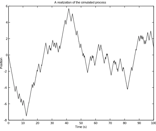
A realization of the simulated process
Time (s)
Position
Figure 2.1: A realization of the simulated process
In Figure 2.1 we can see a realization of the simulated process.
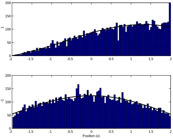
In Figure 2.2, a pair of histograms as approximation of Ψ0xt(x,1) and Ψ1xt(x,1) is shown. There are 20000 data in total used in both histograms. Curves indicating the scaled theoretical density function are also shown. The theoretical density functions are scaled to match the sample size of the simulation.
In Figure 2.3, a pair of histograms as approximation of Ψ0
xt(x,2) and Ψ1xt(x,2) is shown. There are 20000 data in total used in both histograms.
In Figure 2.4, a pair of histograms as approximation of Ψ0
xt(x,5) and Ψ1xt(x,5) is shown. The number of data used is reduced to 10000 in order to reduce the computation time.
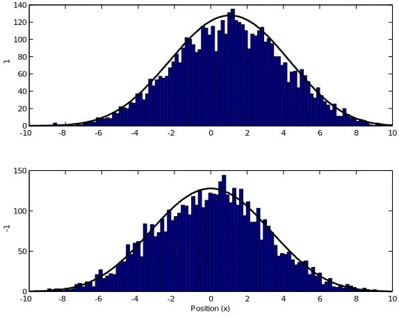
In Figure 2.5, a pair of histograms as approximation ofΨ0
xt(x,10) andΨ1xt(x,10) is shown. The number of data used is also 10000 in total for both histograms.
We can observe that after 1 second, the densityΨ0xt(x,1) is still dominated by the
-1 -0.8 -0.6 -0.4 -0.2 0 0.2 0.4 0.6 0.8 1 0
50 100 150 200
ψ
1
-1 -0.8 -0.6 -0.4 -0.2 0 0.2 0.4 0.6 0.8 1
0 50 100 150 200
Position (x)
ψ
-1
Figure 2.2: Histograms of the state at t = 1. Above : θ1 = 0. Below : θ1 = 1. The
curves represent the scaled theoretical density functions.
-2 -1.5 -1 -0.5 0 0.5 1 1.5 2
0 50 100 150 200
ψ
1
-2 -1.5 -1 -0.5 0 0.5 1 1.5 2
0 50 100 150 200
Position (x)
ψ
-1
Figure 2.3: Histograms of the state at t = 2. Above : θ2 = 0. Below : θ2 = 1. The
-5 -4 -3 -2 -1 0 1 2 3 4 5 0
20 40 60 80 100 120
ψ
1
-5 -4 -3 -2 -1 0 1 2 3 4 5
0 20 40 60 80 100 120
Position (x)
ψ
-1
Figure 2.4: Histograms of the state at t = 5. Above : θ5 = 0. Below : θ5 = 1. The
curves represent the scaled theoretical density functions.
-100 -8 -6 -4 -2 0 2 4 6 8 10
20 40 60 80 100 120 140
ψ
1
-100 -8 -6 -4 -2 0 2 4 6 8 10
50 100 150
Position (x)
ψ
-1
Figure 2.5: Histograms of the state at t= 10.Above : θ10 = 0. Below : θ10 = 1.The
A Model with Di
ff
usion and
Boundary Hitting Process
3.1
Model Formulation
In this chapter we consider a model of linear systems with mode changes triggered by a BHP. The model we use is of the form described below.
Consider a stochastic hybrid system characterized by the following (Ito) SDE.
xt ∈ R
θt ∈ M ={0,1}
ξt , (xt,θt)T
t ∈ R+,
dxt = [a(θt)xt+α(θt)]dt+dWt+b0(θt−)dkt0+b1(θt−)dk1t
dθt = c0(θt−)dkt0+c1(θt−)dk1t (3.1)
where
k0t = Lt(R+)
k1t = Lt(R−) (3.2)
and
θt− = lim
τ↑tθτ
We assume that there exist a probability space (Ω, P,F) and a filtration Ft such that the processξtis adapted to it.
As usual,Wtdenotes a standard Brownian motion. Moreover, we also define
Lt(A) : Ω→{0,1}
Lt =
(
1, if lim s↑txs∈A
0, otherwise (3.3)
a(θ)≤0,∀θ∈M (3.4)
b0(θt−) =
½
0, θt− = 0
1, θt− = 1 (3.5)
b1(θt−) =
½
−1, θt− = 0
0, θt− = 1 (3.6)
c0(θt−) =
½
0, θt− = 0
−1, θt− = 1 (3.7)
c1(θt−) =
½
1, θt− = 0
0, θt− = 1 (3.8)
Throughout this text we will refer to xt, θt, and ξt as the continuous state, discrete state (mode), and hybrid state resp. For the initial condition ξt, we assume that the following relation holds.
(x0,θ0)∈((R+−{0})× {0})∪((R−−{0})× {1}) (3.9) Definition 3.1 As for the previous model, we define the modal density Ψθxt(x, t)such
that for every setΓ in the Borelfield of Rwe have the following relation.
P(xt∈Γ,θt=θ) =
Z
Γ
Ψθxt(x, t)·dx (3.10) We are particularly interested in describing and solving the evolution of Ψ0
xt(x, t) andΨ1
xt(x, t).
Example 3.2 As an example of a process described by (3.1) - (3.9), we define the drift term as in (3.11) below.
[a(0)xt+α(0)] , −1
[a(1)xt+α(1)] , −xt−1. (3.11)
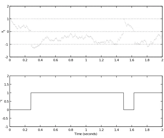
Later in this report, this process will be used as an example for the discussion. A realization of this process is plotted in Figure 3.1. The process depicted here starts at
(x0,θ0) = (1,0). When the process is about to hit the boundary (around t = 0.3 s),
it jumps such that it starts at x = −1 and the mode switches to 1. Again, when the
boundary is about to be hit (aroundt= 1.5s) the process jumps back to the mode 0 and
x= 1.In between the jumps, the process follows the diffusion equation described for the
currently valid mode.
3.2
Di
ff
usion with an Absorbing Boundary
Before we proceed with solving (3.1), we will devote this section for discussion of diffusion with an absorbing boundary. Later it will become clear that the discussion in this section is closely related to the solution of (3.1).
Letxtbe the solution of
dxt=a(x, t)dt+b(x, t)dWt,
0 0.2 0.4 0.6 0.8 1 1.2 1.4 1.6 1.8 2 -2
-1 0 1 2
xt
0 0.2 0.4 0.6 0.8 1 1.2 1.4 1.6 1.8 2
-1 -0.5 0 0.5 1 1.5 2
Time (seconds) θt
Figure 3.1: A realization of a process described by Example 3.2. Top : The continuous state. Bottom : The mode
SDE (refer to e.g. [GS72] and [WH85]). Considering (3.1), for example, we can take
G = {x ∈ R | x > 0) or G = {x ∈ R | x < 0) and ∂G = {0}. We can describe a
diffusion process with absorbing boundary as a phenomenon where upon arrival at a boundary point (state) the process is to remain in that state for all times. In order to give a mathematical representation of such process, let us first consider the following definitions.
Definition 3.3 Thefirst passage timeτx is defined as
τx= inf{t≥0 :xt= 0}
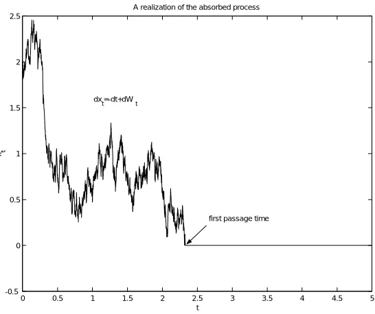
Using the definition ofτx,the absorbed process can be defined as follows.
Definition 3.4 We define the absorbed processx˜t as the stochastic process satisfying ˜
xt=
½
xt, ift <τx
0, ift≥τx (3.12)
with initial condition x˜0=x0.
An example of the realization of an absorbed process is shown in Figure 3.2. Consider the following definition of astopping time.
Definition 3.5 A stopping timeτ for a processxt is a random variable mappingΩ→
(R+∪ ∞)such that the event (τ≤t) is measurable underF
t.
We can notice that τx is a stopping time since the event (τx ≤ t) = (∃s ≤ t :
0 0.5 1 1.5 2 2.5 3 3.5 4 4.5 5 -0.5
0 0.5 1 1.5 2 2.5
A realization of the absorbed process
t
xt
first passage time dx
t=-dt+dWt
Figure 3.2: A realization of an absorbed process
Theorem 3.6 Letxt be the solution of
dxt=a(x, t)dt+b(x, t)dWt,
in an open proper domain G⊂Rwith a smooth boundary ∂G.Define
τx(y, s),inf(t≥s:x(t)∈∂G, x(s) =y). Then the following relation holds true
Eτx(y, s) =s+u(y, t)|t=s, (3.13)
whereu(y, t)is the solution of the following PDE.
∂u
∂t +a(y, t)
∂u
∂y +
1 2b
2(y, t)∂2u
∂y2 =−1, t≥s, y∈G (3.14)
u(y, t) = 0, y∈∂G. (3.15)
Proof. The derivation is given in [Sch80] for the multi dimensional case. It will not be rewritten here.
Theorem 3.7 Letτx(y, s)be defined as in Theorem 3.6, the following relation is also valid.
P(τx(y, s)< T) = q(y, t;T)|t=s,
whereq(y, t, T)is the solution of
∂q
∂t +a(y, t)
∂q
∂y +
1 2b
2(y, t)∂2q
q(y, t;T) = 1, y∈∂G, T ≥t≥s (3.17)
q(y, T;T) = 0, y∈G (3.18)
Proof. The derivation of this theorem is also given in [Sch80].
We will now implement Theorem 3.7 to obtain the density of thefirst passage time for each mode of the process in Example 3.2. We assume that x= 0 is an absorbing boundary. Implementing the theorem to the process described in Example 3.2, we obtain the following relations.
• Ifx0=y >0,
∂q
∂t −
∂q
∂y +
1 2
∂2q
∂y2 = 0, T > t≥0, y >0 (3.19)
q(y, t;T) = 1, y= 0, T ≥t≥0 (3.20)
q(y, T;T) = 0, y >0 (3.21)
• Ifx0=y <0
∂q
∂t −(1 +y)
∂q
∂y +
1 2
∂2q
∂y2 = 0, T > t≥0, y <0 (3.22)
q(y, t;T) = 1, y= 0, T ≥t≥0 (3.23)
q(y, T;T) = 0, y <0 (3.24)
Let us solve the PDE described by (3.19)-(3.21). First, we do the following substi-tution of independent variable.
˜
t,T−t (3.25)
The problem is then transformed into
−∂q
∂˜t −
∂q
∂y+
1 2
∂2q
∂y2 = 0, T ≥˜t >0, y >0 (3.26)
q(y,˜t) = 1, y= 0, T ≥˜t≥0 (3.27)
q(y,˜t) = 0, y >0,˜t= 0 (3.28) Let us define the Laplace transformation ofq(y,t˜;T) in the ˜t direction,
Q(y;s),
Z ∞
0
q(y,˜t)·e−s˜td˜t, (3.29) then using the initial condition (3.28), (3.26) and (3.27) are transformed into the fol-lowing ODE.
−sQ−dQ
dy +
1 2
d2Q
dy2 = 0 (3.30)
Q(0;s) = 1
s (3.31)
Another extra condition can be added, i.e.
The interpretation of (3.32) is clear i.e. the probability of hitting the boundary within the time frame is zero if we start from a point with infinite distance from the boundary. The solution of (3.30) is in the form of
Q(y;s) =C1(s)e(1+ √
1+2s)y+C
2(s)e(1− √
1+2s)y. (3.33)
Imposing the conditions (3.31) and (3.32), we yield
Q(y;s) = e
(1−√1+2s)y
s . (3.34)
After doing inverse transform on (3.34), we will obtain
q(y,˜t) =
Z ˜t
0
y t√2πtexp
µ
−(y−t) 2
2t
dt. (3.35)
Now, regarding Theorem 3.7 and (3.25), we can interpretq(y,˜t) as the probability that the process hits the boundary ˜t time unit after it starts at xt0 = y for any t0 ≥ 0.
Without losing generality, we can sett0= 0.Then the following relation holds true.
P(τx(y,0)<t˜) =q(y,˜t) (3.36) The density functionpτx(y,0)(t) can then be given as
pτx(y,0)(t) =
y t√2πtexp
µ
−(y−t) 2
2t
(3.37) Solving the PDE system (3.22) - (3.24) is more complicated. The results provided below are obtained from modifying the results presented in [Lef96]. The moment gener-ating function of the difference between thefirst passage timeτx(y, s) and the starting timesis given by the following relation
φ(σ, y),E(e−σ(τx(y,s)−s))
This expression is independent ofs.Fory <0,the solutionφ(σ, y) is given by
φ(σ, y) =e(y+1)22 −1 · D−σ
¡
−√2(y+ 1)¢
D−σ
¡
−√2¢ (3.38)
whereD−σ(·) is a parabolic cylinder function called the Weber function. See [MI72] for
more information on this function.
3.3
Solution of Equation (3.1)
We will propose a way to construct the solutionξt.Fori= 1,2,3,· · ·,letˇξit,(ˇxi t,ˇθ
i t)Tbe the solution of
dxˇit = ha(θˇit)xt+α(ˇθ i t)
i
dt+dWt
with initial condition at timet=τi−1 as followsˇξ
i
τi−1 ,(ˇx i
0,ˇθ
i
0)T.We define
τi,inf(t >τi−1:xˇit= 0) (3.40)
withτ0= 0.Notice thatτi is a stopping time.
Let T ∈ R > 0. Define a stochastic process ˇξt whose sample paths in [0, T] are constructed as follows.
1. Letˇξ10=ξ0.
2. Obtain a sample path ofˇξ1t until the stopping timeτ1.
3. Fori= 1,2,3,· · ·,let the initial conditionξˇiτ+1i be determined fromˇξiτi.That is, ˇξi+1
τi = (−1,1)
Tifˇθi
τi= 0,and ˇ
ξiτ+1i = (1,0)T ifˇθi
τi = 1.
4. Start the process ˇξit+1 from the stopping timeτi until the stopping timeτi+1.
5. Repeat step 3 and 4 until a sample path ofˇξNt is obtained whereτN > T. 6. A sample path ofˇξtis obtained by concatenating those ofˇξit,i.e.
ˇ
ξt=ˇξit, fort∈[τi−1,τi) (3.41) Definition 3.8 We define the set JT , {τ1,τ2,τ3,· · · } with 0 = τ0 < τ1 < τ2 <
τ3· · ·≤T.
Remark 3.9 Lett∈[0, T], andξtbe the solution of (3.1) with initial conditionξ0. Let JT ={τ1,τ2,τ3,· · · }with 0 =τ0 <τ1<τ2<τ3· · ·≤T.The state at the jump times
ξτi, i∈Nare actuallyF0−measurable.
The following theorem provides us with the way to characterize a solution of (3.1).
Theorem 3.10 Lett∈[0, T], andˇξtbe the stochastic process as described above. The
process ˇξt is a solution of (3.1) with initial conditionξ0.
Proof. We will show thatˇξs, s∈[0, T] satisfies ˇ
xs=x0+
Z s
0
£
a(ˇθt)ˇxt+α(ˇθt)
¤
dt+
Z s
0
dWt+
Z s
0
b0(ˇθt−)dkt0+
+
Z s
0
b1(ˇθ−t)dk1t (3.42)
ˇ
θt=θ0+
Z s
0
c0(ˇθt−)dkt0+
Z s
0
c1(ˇθt−)dk1t (3.43)
By the nature of the construction of ˇξt we will evaluate the integrals in (3.42) and (3.43) segment by segment. Equivalently, for s ∈[τi,τi+1],∀i∈ {i |i≥ 0,τi+1 ∈ JT} the relations (3.42) and (3.43) can also be written as
ˇ
xs=xˇτi+
Z s
τi
£
a(ˇθt)ˇxt+α(ˇθt)
¤
dt+
Z s
τi
dWt+
Z s
τi
b0(ˇθt−)dkt0+
+
Z s
τi
ˇ
θt=ˇθτi+
Z s
τi
c0(ˇθt−)dkt0+
Z s
τi
c1(ˇθt−)dkt1 (3.45)
It is trivial to verify that the initial condition is satisfied. Moreover, ifs∈[τi,τi+1)
the last two terms of (3.44) and (3.45) evaluate to zero. Hence for s ∈ [τi,τi+1) the
relations (3.44) and (3.45) are satisfied by the construction ofˇξit+1. Ifs=τi+1,it can
also be verified that the jump (i.e. ˇξτ−
i+1 to ˇ
ξτi+1) is consistent with (3.44) and (3.45), as the integral terms involvingdk0
t anddk1t will cover the gap caused by the jump. The verification will be done as follows :
• For the jumps fromˇξτ−
i+1= (0,0) to ˇ
ξτi+1 = (−1,1)
Z τi+1
τ−i+1
b0(ˇθt−)dkt0+
Z τi+1
τ−i+1
b1(ˇθt−)dk1t = 0−1
=−1
Z τi+1
τ−
i+1
c0(ˇθt−)dkt0+
Z τi+1
τ−
i+1
c1(ˇθt−)dk1t = 0 + 1
= 1 • For the jumps fromˇξτ−
i+1= (0,1) to ˇ
ξτi+1 = (1,0)
Z τi+1
τ−i+1
b0(ˇθt−)dkt0+
Z τi+1
τ−i+1
b1(ˇθt−)dk1t = 1 + 0
= 1
Z τi+1
τ−i+1
c0(ˇθt−)dkt0+
Z τi+1
τ−i+1
c1(ˇθt−)dk1t =−1 + 0
=−1 The reader is suggested to refer to Figure 3.1.
Proposition 3.11 Almost every sample path ofˇξit is uniformly continuous in [0, T].
Proof. The proof is based on [GS72]1. It is sufficient if we can show that there
exists a constantK >0 such that
h
a(ˇθit)x+α(ˇθit)i2+ 1≤K2(1 +x2) (3.46)
¯ ¯ ¯a(ˇθit)
¯ ¯
¯≤K (3.47)
For the ease of writing the proof, a(ˇθit) and α(ˇθit) will be simply written as a and α
respectively.
Manipulating (3.46), we obtain
(K2−a2)x2−2aαx+K2−1−α2≥0 (3.48) We then have tofindKsuch that the discriminant of (3.48) is less than zero. In addition, (3.47) is also has to be satisfied. We then get the following relation
4a2α2−4(K2−a2)(K2−1−α2)<0
K4−(a2+α2+ 1)K2+a2>0 (3.49) Notice that the discriminant of (3.49) is
(a2+α2+ 1)2−4a2= (a2+α2+ 1−2a)(a2+α2+ 1 + 2a) = ((a−1)2+α2)·((a+ 1)2+α2)
≥0
which guarantees that (3.49) has real solutions. Letqbe the largest root of (3.49) then choosing
K >max(|a|,pmax(0, q)) will satisfy (3.46) and (3.47), thus completing the proof
Theorem 3.12 Equation (3.1) admits a unique right continuous solution for every ini-tial condition satisfying (3.9).
Proof. It has been shown that the solution can be constructed as piecewise diffu-sions. By construction of the solution and the path continuity ofˇξit, right continuity is established (see Theorem 3.10 and Proposition 3.11). It can be proven that the solutions for the diffusions are unique for each eligible initial condition. In [Oks98] and [GS72] it is stated that if the conditions in the proof of Proposition 3.11 are satisfied then the diffusion admits unique solution.
To show the uniqueness of the whole solution we need to establish the uniqueness of the jumps. But this is more or less trivial since the jumps are constructed such that the states where the process jumps from and where it jumps into are unique for each piece of diffusion. Hence the uniqueness of the solution is established.
3.4
Evolution of Modal Density
Let us introduce the modal transition density.
Definition 3.13 The modal transition density, denoted as Ψθxt|ξ
s(x, t), with s ≤ t,is
the density function such that for any setΓin the Borelfield ofRwe have the following
relation
P(xt∈Γ,θt=θ|ξs) =
Z
Γ Ψθxt|ξ
s(x, t)·dx
We will use the model of diffusion with absorbing boundary to assist us in formulating the evolution of the transition density. First, consider the shifted process (ξ+s)t.
Notation 3.14 The shifted process (ξ+s)t , ξs+t. This notation follows the one in
[BW90]. The continuous and discrete part of the shifted process are then denoted as
(x+
Next, consider the following relations
P(xt∈Γ,θt=θ|ξs) =P((x+s)t−s∈Γ,(θ+s)t−s=θ|(ξ+s)0) (3.50)
P((x+s)t−s∈Γ,(θ+s)t−s=θ|(ξ+s)0) =P((x+s)t−s∈Γ,(θ+s)t−s=θ,τ(x+
s)< t−s|(ξ
+
s)0)
+P((x+s)t−s∈Γ,(θ+s)t−s=θ,τ(xs+)≥t−s|(ξ
+
s)0) (3.51)
Notice that the process definition (3.1) and the limitations on the initial density (3.9) imply that
P(xt ≤ 0,θt= 0) = 0
P(xt ≥ 0,θt= 1) = 0. (3.52)
It is then natural to assume that Γ is strictly contained in either half of R. In the following discussion we will evaluate thefirst term of the right hand side of (3.51).
Proposition 3.15 Given the process described by (3.1), the probability of re-entrance
within a small time interval∆iso(∆), i.e. for allt≥0, the following relation holds.
P(∃s:t < s < t+∆, θt=θt+∆6=θs|ξt) =o(∆)
Proof. The proof is based on the fact that for the re-entrance to occur, the process have to hit the boundary twice. Once the process hit the boundary it will jump to a state away from the boundary so it will have to traverse along a certain distance before hitting the boundary again.
Suppose that
xt=y6= 0
a(θt) =a≤0
α(θt) =α
(3.53)
It has been proved (Theorem 3.10) that the solution of (3.1) can be decomposed such that there is aδ>0,such that ifh <δthe following relation is true.
xt+h=xt+
Z t+h
t
[axτ+α]dτ+Wt+h−Wt
θt+h=θt (3.54)
Consider the process given by (3.54) for all h >0. Now, it can be derived from (3.54) that
xt+h−xt=
³
y+α
a
´
(eah−1) +ea(t+h)
Z t+h
t
e−aτdWτ, a6= 0
xt+h−xt=hα+
Z t+h
t
dWτ, a= 0 (3.55)
We can then have the following relations
E(xt+h−xt|ξt) =
½ ¡
y+αa¢(eah−1), a6= 0
hα, a= 0 (3.56)
sincea(θt)≤0,we have that ¯
We can infer that
|E(xt+h−xt|ξt)|≤(|ay|+|α|)h
= (−a|y|+|α|)h (3.58)
Equation (3.58) implies that for anyy we can choose a limitl(y) such that
h≤l(y) =⇒|E(xt+h−xt|ξt)|≤
y
2 (3.59)
From (3.55) and (3.56) we can obtain
∆h,xt+h−xt−E(xt+h−xt|ξt) =
( Rt+h t e−
a(τ−t−h)dW
τ, a6= 0
Rt+h
t dWτ, a= 0
Now,∆h is a zero mean normal variable, and through the Ito isometry we know that
E(∆2h)≤E(Wt+h−Wt)2=h,∀h >0 (3.60)
Since the solution of (3.54) is continuous (and hence separable), by symmetry we have that
P
µ
sup
0≤s≤h
∆s> |y|
2
=P
µ
inf
0≤s≤h∆s<
−|y|
2
≤P
µ
sup
0≤s≤h
(Wt+s−Wt)> |
y|
2
(3.61) It is known that (see e.g. [GS72]) the following relation holds true
P
µ
sup
0≤s≤h
(Wt+s−Wt)>|
y|
2
= 2P
µ
(Wt+h−Wt)>|
y|
2
≤2h
µ 2
|y|
¶2
= 8h
y2 (3.62)
The inequality above is a Markov inequality. We have the following relation
sup
0≤∆≤h
(|xt+∆−xt|)≤ sup
0≤∆≤h
(|xt+∆−xt|−E(|xt+∆−xt|)) + + sup
0≤∆≤h
(E(|xt+∆−xt|)). (3.63) Now, if we takeh≤l(y) then (3.59), (3.61),(3.62) and (3.63) imply that
P( sup
0≤∆≤h|
xt+∆−xt|≥y|ξt)≤ 8h
y2, (3.64)
and hence
P(the process hits the boundary in [t, t+h]|ξt)≤8h
y2 (3.65)
In order to prove the proposition, it is sufficient if we can show that the following relations hold true.
P(the process hits the boundary in [t, t+∆]|xt=y >0,θt= 0)×
P(the process hits the boundary in [t, t+∆]|xt=y <0,θt= 1)×
×P(the process hits the boundary in [t, t+∆]|xt= 1,θt= 0) =o(∆) (3.67) Notice that (3.66) and (3.67) are upper bounds for the re-entrance probability forxt>0 andxt<0 respectively.
For simplicity, let us denote the left hand sides of (3.66) and (3.67) as X and Y respectively. Then the following relations can be derived through (3.65).
lim ∆↓0
X ∆≤∆lim↓0
1 ∆
8∆
y2
8∆
1 = 0 (3.68)
lim ∆↓0
Y ∆≤lim∆↓0
1 ∆
8∆
y2
8∆
1 = 0 (3.69)
This completes the proof.
Proposition 3.15 indicates that if we want to analyze the variation of the modal density in a small time interval, we can assume that there is only one boundary hitting event in such an interval.
Notation 3.16 Recall the definition of the stopping timesτi in 3.3. We introduce the
following notation,
τs<,τν−s, whereν ,min
i≥0(i|τi> s).
In other words,τs< denotes the time difference between sand thefirst jump time after
s.
Proposition 3.17 Consider the process described by (3.1). Assume that s ≥ 0 and
∆>0.Given Ψ0
xt(x, s) andΨ1xt(x, s),under assumption that at most one jump occurs
in [s, s+∆], the following relations hold true.
Ψ0xt(x, s+∆) =ψ0,0(x;s,∆) +ψ0,1(x;s,∆) (3.70a) Ψ1xt(x, s+∆) =ψ1,1(x;s,∆) +ψ1,0(x;s,∆) (3.70b)
whereψ0,0(x;s,∆)≡ p0(x, t)¯¯
t=s+∆ is the solution of the PDE
∂p0
∂t −
1 2
∂2p0
∂x2 +∂∂x
¡
[a(0)x+α(0)]p0¢= 0
p0(x, s) =Ψ0
xt(x, s)
p0(0, t) = 0
x >0, t > s
, (3.71)
andψ1,1(x;s,∆)≡p1(x, t)¯¯
t=s+∆ is the solution of the PDE
∂p1
∂t −
1 2
∂2p1
∂x2 +∂∂x
¡
[a(1)x+α(1)]p1¢= 0
p1(x, s) =Ψ1xt(x, s)
p1(0, t) = 0
x <0, t > s
. (3.72)
The other two terms are defined as
ψ0,1(x;s,∆) =
Z ∆
0
q0(x,∆−r)·pτ1
s<(r)dr (3.73a)
ψ1,0(x;s,∆) =
Z ∆
0
q1(x,∆−r)·pτ0
The densitiespτ0
s<(·)andpτ1s<(·)are defined as follows. For anyτ >0,
P(τs<≤τ,θs= 0 ),
Z τ
0
pτ0
s<(r)dr (3.74a)
P(τs<≤τ,θs= 1 ),
Z τ
0
pτ1
s<(r)dr (3.74b)
The functions q0(x, t)andq1(x, t) are defined as the solutions of the following PDEs
∂q0
∂t −
1 2
∂2q0
∂x2 +∂∂x
¡
[a(0)x+α(0)]q0¢= 0
q0(x,0) =δ(x−1)
q0(0, t) = 0
x >0, t >0
(3.75)
∂q1
∂t −
1 2
∂2q1
∂x2 +∂∂x
¡
[a(1)x+α(1)]p1¢= 0
q1(x,0) =δ(x+ 1)
q1(0, t) = 0
x <0, t >0
. (3.76)
Proof. Due to symmetry, the proof will be given for half of the proposition i.e. the part related to (3.70a), (3.71), (3.73a), (3.96), and (3.75). The other half will follow the same line.
We start with the following relation forΓ⊂R+.
P(xs+∆∈Γ,θs+∆= 0) =
=P(xs+∆∈Γ,θs+∆= 0,θs= 0) +P(xs+∆∈Γ,θs+∆= 0,θs= 1). (3.77) Let us define density functions for each term of the right hand side of (3.77), such that
P(xs+∆∈Γ,θs+∆= 0,θs= 0)≡
Z
Γ
ψ0,0(x;s,∆)dx (3.78)
P(xs+∆∈Γ,θs+∆= 0,θs= 1)≡
Z
Γ
ψ0,1(x;s,∆)dx (3.79) Then (3.77) can be written as
Z
Γ Ψ0
xt(x, s+∆)dx=
Z
Γ
ψ0,0(x;s,∆)dx+
Z
Γ
ψ0,1(x;s,∆)dx. (3.80) Since (3.80) is valid for allΓ⊂R+,then we have (3.70a). Notice that since at most one
jump can occur in [s, s+∆], we have the following relation
P(xs+∆∈Γ,θs+∆= 0|θs= 0, xs=y >0) =
=P(xs+∆∈Γ,θs+t= 0,∀t∈[0,∆]|θs= 0, xs=y >0) (3.81) To prove thatψ0,0(x;s,∆) satisfies (3.71), we introduce another densityψ0(x;xs, s,∆) such that
P(xs+∆∈Γ,θs+t= 0,∀t∈[0,∆]|θs= 0, xs=y >0)≡
Z
Γ
In [BW90], it is given that ψ0(x;y, s,∆)≡ p˜0(x, t;y)¯¯t=s+∆ is the solution of the PDE
∂p˜0
∂t −
1 2
∂2p˜0
∂x2 +
∂ ∂x
¡
[a(0)x+α(0)]p0¢= 0
˜
p0(x, s;x
s) =δ(x−y) ˜
p0(0, t;y) = 0
x >0, t > s
, (3.83)
Now, we also have that
P(xs+∆∈Γ,θs+∆= 0,θs= 0) = =
Z ∞
0
Ψ0xt(y, s)·P(xs+∆∈Γ,θs+∆= 0|θs= 0, xs=y)dy. (3.84) Using (3.78) and (3.82) we can obtain
Z
Γ
ψ0,0(x;s,∆)dx=
Z ∞
0
Ψ0xt(y, s)
µZ
Γ
ψ0(x;y, s,∆)dx
dy, (3.85)
which is a Chapman-Kolmogorov equation. By exchanging the order of integration on the right hand side, we obtain
Z
Γ
ψ0,0(x;s,∆)dx=
Z
Γ
Z ∞
0
Ψ0xt(y, s)ψ0(x;y, s,∆)dydx
hence
ψ0,0(x;s,∆) =
Z ∞
0
Ψ0xt(y, s)·ψ0(x;y, s,∆)dy. (3.86)
Defining thatψ0,0(x;s,∆)≡p0(x, t)¯¯
t=s+∆,we get
p0(x, t) =
Z ∞
0
Ψ0xt(y, s)·p˜0(x, t;y)dy, s+∆≥t > s (3.87) Now, notice that ˜p0(x, t;xs) is the Green’s function of the PDE (3.83), hence (3.87)
implies that p0(x, t) is the solution of the same PDE with Ψ0
xt(x, s) as a boundary condition. This proves (3.71).
To prove that ψ0,1(x;s,∆) is characterized by (3.73a), (3.74a), and (3.75) we use the following relation
P(xs+∆∈Γ,θs+∆= 0|θs= 1, xs=y <0) = =
Z r=∆
r=0
P(xs+∆∈Γ,θs+∆= 0,τs<∈[r, r+dr]|θs= 1, xs=y <0). (3.88) Using the Chapman-Kolmogorov equation, we can get (see (3.84))
P(xs+∆∈Γ,θs+∆= 0,θs= 1) = =
Z 0
−∞
Ψ1xt(y, s)·P(xs+∆∈Γ,θs+∆= 0|θs= 1, xs=y <0)dy (3.89) We also have that
P(xs+∆∈Γ,θs+∆= 0,τs<∈[r, r+dr]|θs= 1, xs=y <0) = =P(τs<∈[r, r+dr]|θs= 1, xs=y <0)×
Notice that by the assumption that there can be at most one jump in [s, s+∆] the following relation holds true
P(xs+∆∈Γ,θs+∆= 0|θs= 1, xs=y <0,τs<∈[r, r+dr]) =
=P(xs+∆∈Γ,θs+t= 0,∀t∈[r,∆]|θs= 1, xs=y <0,τs<∈[r, r+dr]) (3.91) We introduce the following compact notation
pτs<|ξs(y, r; 1),pτs<|xs=y,θs=1(r) It is clear by the definition ofpτs<|ξs(y, r; 1) that
P(τs<∈[r, r+dr]|θs= 1, xs=y <0) =pτs<|ξs(y, r; 1)dr (3.92) Moreover, if we define a function densityq0(x, t) such that
P(xs+∆∈Γ,θs+t= 0,∀t∈[r,∆]|θs= 1, xs=y <0,τs<∈[r, r+dr]) = =
Z
Γ
q0(x,∆−r)dx, (3.93) it is known from [BW90] thatq0(x, t) will satisfy (3.75). Now (3.89) can be written as
Z
Γ
ψ0,1(x;s,∆)dx=
Z 0
−∞
Ψ1xt(y, s)
Z ∆
0
µZ
Γ
q0(x,∆−r)dx
·pτs<|ξs(y, r; 1)drdy. (3.94) Exchanging the order of integration, we can obtain
Z
Γ
ψ0,1(x;s,∆)dx=
Z
Γ
Z ∆
0
Z 0
−∞
q0(x,∆−r)·Ψ1xt(y, s)·pτs<|ξs(y, r; 1)dydrdx =
Z
Γ
Z ∆
0
q0(x,∆−r)·pτ1
s<(r)drdx (3.95) We use Lemma 3.18 to derive the second line of (3.95). Since (3.95) is valid for all Γ⊂R+,we obtain (3.73a).
Lemma 3.18 Letpτs<|ξs(x, t;θ)be the distribution density ofτs< given(xs=x,θs=
θ),such that for anyτ>0
P(τs<≤τ|xs=x,θs=θ)≡
Z τ
0
pτs<|ξs(x, t;θ)dt
then, by referring to (3.74a) and (3.74b), the following relations hold true,
pτ0 s<(r) =
Z ∞
0
Ψ0xt(x, s)·pτs<|ξs(x, r; 0)dx (3.96)
pτ1 s<(r) =
Z 0
−∞
Ψ1xt(x, s)·pτs<|ξs(x, r; 1)dx (3.97)
Proof. By symmetry, only (3.96) will be proven. Referring to (3.74a), we have that for anyτ >0,
P(τs<≤τ,θs= 0),
Z τ
0
But we also have that
P(τs<≤τ,θs= 0) =
Z
y∈R+
P(τs<≤τ, xs∈[y, y+dy],θs= 0) =
Z
y∈R+
P(τs<≤τ|xs∈[y, y+dy],θs= 0)×P(xs∈[y, y+dy],θs= 0) =
Z
y∈R+
Z τ
0
pτs<|ξs(y, r; 0)dr·Ψ
0
xs(y)dy (3.99)
By exchanging the order of integration, we obtain
P(τs<≤τ,θs= 0) =
Z τ
0
Z
y∈R+
pτs<|ξs(y, r; 0)Ψ
0
xs(y)dydr. (3.100)
Finally, by comparing (3.100) and (3.74a) we obtain (3.96).
Theorem 3.19 The densitiesΨ0
xt(x, t) andΨ1xt(x, t)satisfy the following PDEs
∂Ψ0 xt
∂t =
1 2
∂2Ψ0 xt
∂x2 −∂∂x
¡
[a(0)x+α(0)]Ψ0
xt
¢
+pτ1
t<(0)·δ(x−1) Ψ0
xt(x,0) =Ψ0x0(x) Ψ0
xt(0, t) = 0
x >0, t≥0
(3.101)
∂Ψ1xt
∂t =
1 2
∂2Ψ1xt
∂x2 −∂∂x
¡
[a(1)x+α(1)]Ψ1
xt
¢
+pτ0
t<(0)·δ(x+ 1) Ψ1
xt(x,0) =Ψ1x0(x) Ψ1
xt(0, t) = 0
x <0, t≥0
(3.102)
whereΨ0
x0(x)andΨ1x0(x)are the densities of the initial condition.
Proof. Refer to Proposition 3.17. For anys≥0,we have that Ψ0xt(x, s+∆)−Ψ0xt(x, s)
∆ =
ψ0,0(x;s,∆)−Ψ0xt(x, s)
∆ +
ψ0,1(x;s,∆)
∆ . (3.103)
By taking the limit of∆↓0,we obtain
∂Ψ0
xt
∂t
¯ ¯¯ ¯
t=s = lim
∆↓0
ψ0,0(x;s,∆)−Ψ0
xt(x, s) ∆ + lim∆↓0
ψ0,1(x;s,∆)
∆ (3.104)
Referring to (3.71), we see that lim
∆↓0
ψ0,0(x;s,∆)−Ψ0
xt(x, s)
∆ =
∂ψ0,0(x;s,∆)
∂∆ ¯ ¯ ¯ ¯ ∆=0 = = ∂p
0
∂t
¯ ¯ ¯ ¯t=s=
1 2
∂2Ψ0
xt
∂x2 +
∂ ∂x
¡
[a(0)x+α(0)]Ψ0xt¢. (3.105) We also have that (see (3.73a))
lim ∆↓0
ψ0,1(x;s,∆) ∆ = lim∆↓0
1 ∆
Z ∆
0
q0(x, s+∆−r)·pτ1 s<(r)dr =q0(x, s)·pτ1
s<(0) =δ(x−1)·pτ1
Proving the boundary conditions in (3.101) is more or less trivial since they can be derived easily from those of (3.71) and (3.75). Hence, from (3.105) and (3.106) we can obtain (3.101).
Following the same line we can derive for anys≥0
∂Ψ1xt
∂t = lim∆↓0
ψ1,1(x;s,∆)−Ψ1xt(x, s) ∆ + lim∆↓0
ψ1,0(x;s,∆)
∆ . (3.107)