An explicit construction of fast cocyclic jacket transform on the finite field with any size

R E S E A R C H

Open Access

An explicit construction of fast cocyclic jacket

transform on the finite field with any size

Ying Guo

, Moon Ho Lee

and Kyeong Jin Kim

Abstract

An orthogonal cocyclic framework of the block-wise inverse Jacket transform (BIJT) is proposed over the finite field. Instead of the conventional block-wise inverse Jacket matrix (BIJM), we investigate the cocyclic block-wise inverse Jacket matrix (CBIJM), where the high-order CBIJM can be factorized into the low-order sparse CBIJMs with a successive block architecture. It has a recursive fashion that leads to a fast algorithm concerned for reducing computational load. The fast transforms are also developed for the two-dimensional cocyclic block-wise inverse Jacket transform (CBIJT). The present CBIJM may be used for many matrix-based applications, such as the DFT signal processing, combinatorics, and the Reed-Muller code design.

Introduction

The orthogonal transforms, such as the discrete Fourier transform (DFT) and the Walsh-Hadamard transform (WHT), have been widely employed in images process-ing, feature selection, signal processprocess-ing, data compressing and coding, and other areas [1-7]. Using orthogonality of the WHT, the interesting orthogonal matrices, such as the element-wise or block-wise inverse Jacket matrices (BIJMs) [8-12], have been developed. More details of these matrices can be referred to [13-19].

Definition 1.Ann×nmatrixJn = (αij)n×nis called the element-wise inverse Jacket matrix (EIJM) of order n if its inverse matrix J_n−1 can be simply obtained by its element-wise inverse, i.e.,J_n−1 = _n1(α_ij−1)T_n×n,∀ i,j ∈ Zn := {0, 1,. . .,n−1}, where the superscript T denotes the transpose.

Many interesting orthogonal matrices, say the

Hadamard matrices and the DFT matrices, belong to the Jacket matrix family. With the rapid technological development, different forms of such transforms were improved and generalized. It has been discovered that the

*Correspondence: [email protected]

2Institute of Information and Communication, Chonbuk National University, Jeonju 561-756, Korea

Full list of author information is available at the end of the article

newly proposed transforms have been widely used in var-ious signal processing, CDMA, cooperative relay MIMO system [20-28].

Recently, the BIJM [J]nhas been investigated while the complex unit exp√−1(2π/p) of the EIJM Jn is substituted for a suitable matrix unit [15-17]. However, the CBIJM does not attract much attention even though the cocyclic matrix has been very useful for the data coding and processing [5,14,29,30].

Definition 2.IfGis a finite group of orderrwith oper-ation◦andCis a finite Abelian group of ordert, a cocycle is a mappingφ :G×G→Csatisfying

φ (a,b)φ (a◦b,c)=φ (a,b◦c)φ (b,c), (1) wherea,b,c∈G. A square matrixM(φ)whose rowaand columnbcan be indexed byG with entryφ (a,b) ∈ C in position (a,b) under some fixed ordering, i.e., M(φ) = (φ (a,b))_a,b∈G, is called a cocyclic matrix. Ifφ (1, 1) = 1, then it is the normalized cocyclic matrix for the standard usage [5,29,30].

Definition 3.Let Jp = (ωi◦jp)p×p, ∀ i,j ∈ Zp :=

{0, 1,. . .,p − 1}, be a matrix of order p, where ω = exp(√−1(2π/p))andi◦jp=i×j modp, i.e., the sub-script pimplies modulo-parithmetic for the argument. Then the matrixJpand itss-fold matrix of orderps

Jps =J_p⊗s=J_p⊗J_p· · · ⊗J_p

s

are the conventional cocyclic element-wise inverse Jacket matrices (CEIJM), where⊗denotes the Kronecker prod-uct andpis a prime number.

As a generation of the Hadamard matrix, the BIJM inherits the merits of the Hadamard matrix, at the same time, without the restriction that entries must be ‘±1’. On the other hand, this matrix has very amicable properties, such as reciprocal orthogonality. The inverse transform can be easily obtained by the reciprocal relationships and the fast algorithms. However, the versions of cocyclic block-wise inverse Jacket matrix (CBIJM) are still absent since the existence of the CEIJM has attracted minor attention in the existing literature [8,21]. The purpose of this article is to develop the CBIJM and its general-izations, instead of the CEIJM. In addition, the present CBIJM has some potential practical applications in sig-nal sequence transforms [1-7], coding design for wireless networks [22,27,28], and cryptography [31].

This article is organized as follows. Section ‘Cocyclic block-wise inverse Jacket transforms’ presents a simple framework of the fast CBIJT. Section ‘Designs of the CBIJM over finite field GF(2m)’ reports the CBIJM over finite fieldGF(2p). Section ‘Two-dimensional fast CBIJM’ proposes the structure of the two-dimensional CBIJM. Finally, conclusions are drawn in Section ‘Conclusion’.

Cocyclic block-wise inverse Jacket transforms In this section, we show that the EIJM can be generalized for the constructions of the CBIJT.

Based on the one-dimensional BIJM [J]p of order p, which can be partitioned to the p×pblock matrix, we can transform a suitable vector x into another vectory through a BIJT, i.e.,

y=[J]px. (2)

In order to derive the CBIJT, we denote a matrix unit by αsuch thatαp=Ipfor a given prime numberp, whereIp denotes thep×pidentity matrix. As an example, letαbe a square matrix of size 2×2 defined as

α=

0 1 1 0

. (3)

It is easy to prove thatα2 = I2. Actually, matrixα in (3) has been employed for the existence of the BIJM [15-17]. Fortunately, it will be shown that thes-fold block Jacket matrix [J]2sα⊗sis also a CBIJM.

In what follows we illustrate the cocyclicity of the BIJM [J]psbased on the matrix unitαof sizep×p. In particular

for the given prime numberp, we define the matrix unit αh=[ei,j]p, where

ei,j=

1, for i= j+hp;

0, otherwise, (4)

wherej+hp=j+hmodp,∀i,j,h∈Zp:= {0, 1,. . .,p− 1}. It can be shown thatA := {αh : h ∈ Zp} forms an Abelian group with the traditional matrix multiplication. Namely, for the given numberp, one obtains the matrix units as follows

α0=

⎛ ⎜ ⎜ ⎜ ⎜ ⎜ ⎜ ⎜ ⎝

1 0 0 · · · 0 0 0 1 0 · · · 0 0 0 0 1 · · · 0 0

..

. ... ... ... ... ... 0 0 0 · · · 1 0 0 0 0 · · · 0 1

⎞ ⎟ ⎟ ⎟ ⎟ ⎟ ⎟ ⎟ ⎠

,α1=

⎛ ⎜ ⎜ ⎜ ⎜ ⎜ ⎜ ⎜ ⎝

0 0 0 · · · 0 1 1 0 0 · · · 0 0 0 1 0 · · · 0 0

..

. ... ... ... ... ... 0 0 0 · · · 0 0 0 0 0 · · · 1 0

⎞ ⎟ ⎟ ⎟ ⎟ ⎟ ⎟ ⎟ ⎠

,· · ·

αp−2=

⎛ ⎜ ⎜ ⎜ ⎜ ⎜ ⎜ ⎜ ⎝

0 0 1 · · · 0 0 0 0 0 · · · 0 0 0 0 0 · · · 0 0

..

. ... ... ... ... ... 1 0 0 · · · 0 0 0 1 0 · · · 0 0

⎞ ⎟ ⎟ ⎟ ⎟ ⎟ ⎟ ⎟ ⎠

,αp−1=

⎛ ⎜ ⎜ ⎜ ⎜ ⎜ ⎜ ⎜ ⎝

0 1 0 · · · 0 0 0 0 1 · · · 0 0 0 0 0 · · · 0 0

..

. ... ... ... ... ... 0 0 0 · · · 0 1 1 0 0 · · · 0 0

⎞ ⎟ ⎟ ⎟ ⎟ ⎟ ⎟ ⎟ ⎠

.

(5)

Example 1. Letp=3, and we have

α0=

⎛ ⎝1 0 00 1 0

0 0 1

⎞ ⎠,α1=

⎛ ⎝0 0 11 0 0

0 1 0

⎞ ⎠,α2=

⎛ ⎝0 1 00 0 1

1 0 0

⎞ ⎠.

(6)

It is obvious thatZp with the multiplication operation

a·bpis a finite field of orderp. For∀a,x∈Zp, we define an multiplication functionfa(x)overZp, i.e.,

fa(x):= a·xp. (7)

With the aid of the multiplication function fa(x), we define a block matrix of size p×p2 by concatenatingp matricesαhi_{of sizep}×_p,∀_h

i∈Zp, i.e.,

[β] :=αh0,αh1,. . .,αhp−1 ₍₈₎

and hence

[β_a] :=αfa(h0)_,αfa(h1)_{,. . .,α}fa(hp−1)_{. (9)}

Lemma 1.For block matrices [βa] and [βb], ∀a,b ∈ Zp, we have

[β_a]·[β_b]T=

pI, for a+bp=0;

0, for a+bp=0. (10)

Example 2.Let us considerα withp = 2 in (3). It is obvious thatα2=Iis an identity matrix of size 2×2. Let [β]=α0,α1, then we have

[β0]=

α0,α0=

1 0 1 0 0 1 0 1

, (11)

[β₁]=α0,α1=

1 0 0 1 0 1 1 0

. (12)

It is straightforward to show that

[β0]·[β0]T=[β1]·[β1]T=2I2. (13)

Thep-order CBIJM

In [15-17], Lee et al. expanded the EIJM to the BIJM.

Definition 4.An np × np block matrix [J]n=

([αij]p)np×np is called the BIJM of order n if [J]−n1= 1

c([αij]−1)Tnp×np where c is the normalized value and [α_ij]p×pdenotes a matrix unit of sizep×p.

Definition 5.For a given prime number p, let α be a p×pmatrix unit such thatαp=Iand

[β]=α0,α1,. . .,αp−1. (14) Define thep-order BIJM [J]pof sizep2×p2as follows

[J]p:= ⎡ ⎢ ⎢ ⎢ ⎢ ⎢ ⎣

[β0] [β1] [β₂] .. . [β_p−1]

⎤ ⎥ ⎥ ⎥ ⎥ ⎥

⎦=

⎡ ⎢ ⎢ ⎢ ⎢ ⎢ ⎣

α0 α0 · · · α0 α0 α1 · · · αp−1 α0 α2 · · · α2(p−1)

..

. ... . .. ... α0αp−1 · · ·α(p−1)(p−1)

⎤ ⎥ ⎥ ⎥ ⎥ ⎥ ⎦

(15)

and thus its inverse

[J]−_p1:= 1 p

⎡ ⎢ ⎢ ⎢ ⎢ ⎢ ⎣

α0 α0 · · · α0 α0 α−1p · · · _α−(p−1)p α0 α−2p · · · _α−2(p−1)

..

. ... . .. ...

α0α−(p−1)p· · ·_α−(p−1)(p−1)p

⎤ ⎥ ⎥ ⎥ ⎥ ⎥ ⎦

. (16)

Consequently, we have

[J]p·[J]p−1=[J]p−1·[J]p=Ip2_×p2. (17)

Example 3.Taking [β0] and [β1] forp=2, we have

[J]2=

α0 α0 α0 α1

=

⎡ ⎢ ⎢ ⎣

1 0 1 0 0 1 0 1 1 0 0 1 0 1 1 0

⎤ ⎥ ⎥

⎦, (18)

and its inverse

[J]−₂1= 1 2

α0 α0 α0 α−12

= 1 2

⎡ ⎢ ⎢ ⎣

1 0 1 0 0 1 0 1 1 0 0 1 0 1 1 0

⎤ ⎥ ⎥

⎦. (19)

Actually, we have

[J]2[J]−21=

α0 α0 α0 α1

α0 α0 α0 α1

=

I2 0 0 I2

, (20)

whereα0+α1=0 sinceα2=Iandα=Iover the finite field.

We note that the above-mentioned BIJM was first pro-posed by Lee and Hou [13] for the proof of existence of Jacket matrices over the finite field. Next, we illustrate that this BIJM is also a CBIJM in essence.

Theorem 1.LetG = Zp with an operationa◦b :=

a+bp,∀a,b∈Zp, andC:= {αi :i∈Zp}with the tra-ditional multiplication. The BIJM [J]pin (15) whose rows and columns are both indexed inGunder the increasing order (i.e., 0 ≺ 1 ≺ · · · ≺ p−1) and entriesφ (a,b) in position(a,b)is the normalized CBIJM.

The proof of Theorem 1 is illustrated in Appendix.

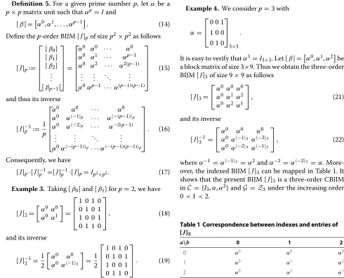
Example 4.We considerp=3 with

α=

⎡ ⎢ ⎣

0 0 1 1 0 0 0 1 0

⎤ ⎥ ⎦

3×3 .

It is easy to verify thatα3=I3×3. Let [β]=

α0,α1,α2be a block matrix of size 3×9. Thus we obtain the three-order BIJM [J]3of size 9×9 as follows

[J]3=

⎡

⎣α

0 _α0 _α0 α0 α1 α2 α0 α2 α1

⎤

⎦, (21)

and its inverse

[J]−₃1=

⎡ ⎣α

0 _α0 _α0 α0 α−13 _α−23 α0 α−23 _α−13

⎤

⎦, (22)

whereα−1= α−13 =_α2_andα−2= _α−23 = _α. More-over, the indexed BIJM [J]3can be mapped in Table 1. It shows that the present BIJM [J]3is a three-order CBIJM inC = {I3,α,α2}andG= Z3under the increasing order 0≺1≺2.

Table 1 Correspondence between indexes and entries of [J]3

a_\b 0 1 2

0 α0 _α0 _α0

1 α0 _α1 _α2

The multi-fold CBIJM

In order to derive the high-order recursive CBIJM [J]ps for any prime numberpand nonnegative integers, let us introduce some lemmas [1-5].

Lemma 2.LetA,B,C, andDare matrices with suitable sizes. Then we have

(A⊗B)·(C⊗D)=(A·C)⊗(B·D), (A⊗B)−1=(A−1⊗B−1),

(A⊗B)T=(AT⊗BT). (23)

Theorem 2. For a given prime number p, let [A]p= [αi,j]pand [B]p=[γs,t]p,∀i,j,s,t∈Zp, be two CBIJMs of orderpthat corresponds to the matrix unitsαandγ such thatαp = Iandγp = I, respectively. Then the two-fold Kronecker product matrix

[J]_p2=[A]p⊗[B]p (24)

is a two-fold CBIJM of orderp2.

The proof of Theorem 2 is shown in Appendix.

Corollary 1.For any prime numberpand non-negative integer number s, let [J]ps=[J]⊗_ps be an s-fold block matrix, i.e.,

[J]ps=[J]_p⊗ · · ·[J]_p

s

. (25)

Then the block matrix [J]psis a CBIJM of orderps.

Example 5.Forp= 2 ands= 2, we consider a matrix unitα of size 2×2 in (3). Thus we have the four-order BIJM [J]₂2given by

[J]₂2 =[J]2⊗[J]2

=

α0 α0 α0 α1

4×4

⊗

α0 α0 α0 α1

4×4

=

⎡ ⎢ ⎢ ⎣

α0α0 α0α0 α0α0 α0α0 α0α0 α0α1 α0α0 α0α1 α0α0 α0α0 α1α0 α1α0 α0α0 α0α1 α1α0 α1α1

⎤ ⎥ ⎥ ⎦

8×8

. (26)

Similarly, we have an index order matrix in Table 2, where the row and column index orders are

00≺01≺10≺11 (27)

and for∀a1,b1,a2,b2∈Z2,

a1a2◦b1b2= a1+b12a2+b22. (28)

As an example, ifa=2 andb=3, then we have

α10◦11=α1+120+12 =_α01=_α.

Table 2 Correspondence between indexes and entries of the2-fold CBIJM [J]22based on the basic CBIJM [J]2

a\b ◦ 00 01 10 11

◦ a\b 0 1 2 3

00 0 α0α0 α0α0 α0α0 α0α0

01 1 α0α0 α0α1 α0α0 α0α1

10 2 α0α0 α0α0 α1α0 α1α0

11 3 α0α0 α0α1 α1α0 α1α1

It can be easily verified that the two-fold matrix [J]₂2 in (26) is a four-order CBIJM of size 8×8. In addition, using the same index mapping in Table 1, we obtain the index matrixI4as follows

I4=

⎡ ⎢ ⎢ ⎣

0 0 0 0 0 1 0 1 0 0 1 1 0 1 1 0

⎤ ⎥ ⎥

⎦, (29)

which is a generator matrix of the first order binary Reed-Muller code [3]. We note that this phenomena exists in the generalizeds-fold CBIJM [J]ps of orderpsfor any prime numberp.

Actually, the two-fold CBIJM [J]₂2in (26) based on the factorization algorithm can be rewritten as

[J]₂2=[J]2⊗[J]2=(I2⊗[J]2) ([J]2⊗I2). (30)

Namely, we have

[J]₂2 = ⎡ ⎢ ⎢ ⎣

α0 α0 α0 α0 α0 α1 α0 α1 α0 α0 α1 α1 α0 α1 α1 α0

⎤ ⎥ ⎥ ⎦

=

⎡ ⎢ ⎢ ⎣

α0 α0 0 0 α0 α1 0 0 0 0 α0 α0 0 0 α0 α1

⎤ ⎥ ⎥ ⎦

⎡ ⎢ ⎢ ⎣

α0 0 α0 0 0 α0 0 α0 α0 0 α1 0

0 α0 0 α1

⎤ ⎥ ⎥ ⎦.

The comparison between the direct computation and fast transform in terms of operations (i.e., additions and mul-tiplications) is illustrated in the Table 3. From this table, it is shown that forN = 4 if we compute directly there are 12 additions and 16 multiplications, but if we use the fast transform algorithm the numbers of additions and multiplications can be reduced to 8 and 4, respec-tively. It is obvious that the proposed algorithm has a

Table 3 Complexity of the fast algorithms forN=ps, where ADD and MUL denote additions and multiplications

Direction method Fast algorithms

ADD (N−1)N sps_(p−1)

greater efficiency for computation than that of the direct approach.

Example 6.From Equation (23), we havep= 3,s= 2 and

α0=

⎡ ⎣1 0 00 1 0

0 0 1

⎤ ⎦,α1=

⎡ ⎣0 0 11 0 0

0 1 0

⎤ ⎦,α2=

⎡ ⎣0 1 00 0 1

1 0 0

⎤ ⎦,

then we can derive the two-fold CBIJM [J]₃2=[J]3⊗[J]3, i.e.,

[J]₃2= ⎡ ⎢ ⎢ ⎢ ⎢ ⎢ ⎢ ⎢ ⎢ ⎢ ⎢ ⎢ ⎢ ⎣

α0 α0 α0 α0 α0 α0 α0 α0 α0 α0 α1 α2 α0 α1 α2 α0 α1 α2 α0 α2 α1 α0 α2 α1 α0 α2 α1 α0 α0 α0 α1 α1 α1 α2 α2 α2 α0 α1 α2 α1 α2 α0 α2 α0 α1 α0 α2 α1 α1 α0 α2 α2 α1 α0 α0 α0 α0 α2 α2 α2 α1 α1 α1 α0 α1 α2 α2 α0 α1 α1 α2 α0 α0 α2 α1 α2 α1 α0 α1 α0 α2

⎤ ⎥ ⎥ ⎥ ⎥ ⎥ ⎥ ⎥ ⎥ ⎥ ⎥ ⎥ ⎥ ⎦

27×27 , (31)

which can be factorized as

[J]₃2=[J]3⊗[J]3=(I3⊗[J]3)([J]3⊗I3)

= ⎡ ⎢ ⎢ ⎢ ⎢ ⎢ ⎢ ⎢ ⎢ ⎢ ⎢ ⎢ ⎢ ⎣

α0 α0 α0 0 0 0 0 0 0

α0 α1 α2 0 0 0 0 0 0

α0 α2 α1 0 0 0 0 0 0

0 0 0 α0 α0 α0 0 0 0

0 0 0 α0 α1 α2 0 0 0

0 0 0 α0 α2 α1 0 0 0

0 0 0 0 0 0 α0 α0 α0

0 0 0 0 0 0 α0 α1 α2

0 0 0 0 0 0 α0 α2 α1

⎤ ⎥ ⎥ ⎥ ⎥ ⎥ ⎥ ⎥ ⎥ ⎥ ⎥ ⎥ ⎥ ⎦

27×27

× ⎡ ⎢ ⎢ ⎢ ⎢ ⎢ ⎢ ⎢ ⎢ ⎢ ⎢ ⎢ ⎢ ⎣

α0 0 0 α0 0 0 α0 0 0

0 α0 0 0 α0 0 0 α0 0

0 0 α0 0 0 α0 0 0 α0

α0 0 0 α1 0 0 α2 0 0

0 α0 0 0 α1 0 0 α2 0

0 0 α0 0 0 α1 0 0 α2

α0 0 0 α2 0 0 α1 0 0

0 α0 0 0 α2 0 0 α1 0

0 0 α0 0 0 α2 0 0 α1

⎤ ⎥ ⎥ ⎥ ⎥ ⎥ ⎥ ⎥ ⎥ ⎥ ⎥ ⎥ ⎥ ⎦

27×27

. (32)

with the signal flow graph in Figure 1. It is obvious that I3⊗[J]3 and [J]3⊗I3 are both sparse matrices, and the two-fold matrix [J]₃2is a nine-order CBIJM of size 27×27. The index matrixI9of [J]32is given by

3-point PE X1 X2 X3 X4 X5 X6 X7 X8 X9 Y1 Y2 Y3 Y4 Y5 Y6 Y7 Y9 Y8

Figure 1Signal flow graph for the two-fold CBIJM[J]32of order nine.

I9=

⎡ ⎢ ⎢ ⎢ ⎢ ⎢ ⎢ ⎢ ⎢ ⎢ ⎢ ⎢ ⎢ ⎣

0 0 0 0 0 0 0 0 0 0 1 2 0 1 2 0 1 2 0 2 1 0 2 1 0 2 1 0 0 0 1 1 1 2 2 2 0 1 2 1 2 0 2 0 1 0 2 1 1 0 2 2 1 0 0 0 0 2 2 2 1 1 1 0 1 2 2 0 1 1 2 0 0 2 1 2 1 0 1 0 2

⎤ ⎥ ⎥ ⎥ ⎥ ⎥ ⎥ ⎥ ⎥ ⎥ ⎥ ⎥ ⎥ ⎦

9×9

which can be used for the generalization of the first order 3-ary Reed-Muller code [3].

Consequently, thes-fold CBIJM [J]ps of orderpscan be generated from the following factorization algorithm

[J]ps=[J]_ps−1⊗[J]p= s

i=1

I_ps−i⊗[J]_p⊗I_pi−1 (33)

whereI_pi denotes the identity matrix of sizepi×pi and I_p0 =1 for the simple description.

Corollary 2.Based on thep-order CBIJM [J]pfor any number p, the s-fold CBIJM [J]ps of order ps can be constructed with the recursive formula

[J]ps= s

i=1

I_ps−i⊗[J]_p⊗I_pi−1 , (34)

where p is any prime number and s is a nonnegative integer number.

In order to show the factorization of the generalized CBIJM [J]n of order ps with any prime number p, we propose several construction approaches in Table 4. In this table, the second column is the decomposition for the numbers (order) of the CBIJM, and the third column is the construction for CBIJM. It shows that the large-order CBIJM can be designed on the basis of the lower order CBIJM [J]p with sparse matrices in the successive architecture.

Low-density of the CBIJM

In what follows, we consider the density of 1’s in thes-fold CBIJM [J]ps.

According to the afore-mentioned CBIJM [J]p, it is known that matrix [J]pwhose matrix unit isαin (4) is a

p2×p2binary matrix. The total number of 1’s ispin each matrix unitαh,∀h∈Zp. Then the density of 1’s inαhis

ρ(αh)= p p2 =

1

p. (35)

Therefore the density of 1’s in [J]pis calculated as

ρ([J]p)=ρ(αh)= 1

p, (36)

and the density of 1’s in thes-fold matrix [J]psis

ρ([J]ps)=ρ([J]_p)= 1

p, (37)

which shows that the larger matrix order p means the lower density of 1’s in both [J]pand [J]ps.

As an example, we consider the CBIJM [J]2in Example 3 and the two-fold CBIJM [J]₂2 in Example 5 with matrix

Table 4 Decompositions of orders for the CBIJM [J]pswith density1/p

Order Decomposition CBIJM Density

2 2=2 [J]2=[J]2 1/2

3 3=3 [J]3=[J]3 1/3

4 22_{=2×2 [J]}

4=[J]⊗22 1/2

5 5=5 [J]5=[J]5 1/5

7 7=7 [J]7=[J]7 1/7

8 23=22×2 [J]8=[J]⊗23 1/2

9 32=3×3 [J]9=[J]⊗32 1/3 11 11₌11 [J]11=[J]11 1/11

13 13₌13 [J]13=[J]13 1/13

16 24₌₂3_{×2 [J]}

16=[J]⊗24 1/2 17 17=17 [J]17=[J]17 1/17

19 19=19 [J]19=[J]19 1/19

23 23=23 [J]23=[J]23 1/23

25 52_{=5×5 [J]}

25=[J]⊗52 1/5

unitα = [ei,j]_2×2in (4). It is easy to verify that the den-sities of 1’s in [J]2, and [J]22 are all 1/2, i.e.,ρ([J]₂2) = ρ([J]2)=1/2. Generally, for any prime numberpwe have ρ([J]_p2)=ρ([J]p)=ρ(α)=1/p, as shown in Table 5.

Designs of the CBIJM over finite field GF(2m) In this section, we consider the generalized CBIJM over finite field GF(2m)and derive the high-order CBIJM for p=2m−1.

Letαbe a matrix unit of sizep×pover GF(2m)such that α2m−1=Iandα=I. Then we obtain the(2m−1)-order CBIJM [J]2m₋₁as follows.

Theorem 3.Let

[J]2m₋₁[_αij]₂m₋₁

be a(2m −1)-order block matrix over GF(2m), ∀ i,j ∈ Z2m₋₁, whereαis a matrix unit of size(2m−1)×(2m− 1)satisfyingα2m−1 = I andα = I. Then block matrix [J]2m₋₁is a CBIJM.

The proof of Theorem 3 are shown in Appendix.

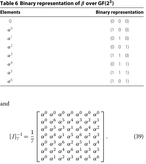
Example 7. We consider the seven-order block matrix [J]₂3₋₁with the primitive polynomialx3+x+1=0 over GF(23). Letαbe an arbitrary matrix unit such thatα7=I andα=I. Then any matrix elementβover GF(23)can be represented as a binary vector(b0,b1,b2),∀bi ∈ Z2and i∈ {0, 1, 2}, such that

β=b0+b1α+b2α2.

By the Table 6, it is straightforward that Theorem 3 is true over GF(23). Then we obtain the BIJM [J]7 and its inverse [J]−₇1, i.e.,

[J]7=

⎡ ⎢ ⎢ ⎢ ⎢ ⎢ ⎢ ⎢ ⎢ ⎣

α0 α0 α0 α0 α0 α0 α0 α0 α1 α2 α3 α4 α5 α6 α0 α2 α4 α6 α1 α3 α5 α0 α3 α6 α2 α5 α1 α4 α0 α4 α1 α5 α2 α6 α3 α0 α5 α3 α1 α6 α4 α2 α0 α6 α5 α4 α3 α2 α1

⎤ ⎥ ⎥ ⎥ ⎥ ⎥ ⎥ ⎥ ⎥ ⎦

, (38)

Table 5 Densities of the matrix unitsα, CBIJM[J]p, and

s-fold CBIJM[J]ps

2 3 5 7 11

α 1/2 1/3 1/5 1/7 1/11

[J]p 1/2 1/3 1/5 1/7 1/11

Table 6 Binary representation ofβover GF(23₎

Elements Binary representation

0 (0 0 0)

α0 (1 0 0)

α1 _{(0 1 0)}

α2 _{(0 0 1)}

α3 _{(1 1 0)}

α4 _{(0 1 1)}

α5 _{(1 1 1)}

α6 (1 0 1)

and

[J]−₇1= 1 7

⎡ ⎢ ⎢ ⎢ ⎢ ⎢ ⎢ ⎢ ⎢ ⎣

α0 α0 α0 α0 α0 α0 α0 α0 α6 α5 α4 α3 α2 α1 α0 α5 α3 α1 α6 α4 α2 α0 α4 α1 α5 α6 α2 α3 α0 α3 α6 α2 α5 α1 α4 α0 α2 α4 α6 α1 α3 α5 α0 α1 α2 α3 α4 α5 α6

⎤ ⎥ ⎥ ⎥ ⎥ ⎥ ⎥ ⎥ ⎥ ⎦

. (39)

Actually, according to the index mapping of the present matrix in Table 7, it can be shown that matrix [J]7in (38) is a seven-order CBIJM over GF(23_).

Two-dimensional fast CBIJM

In the previous section, we consider the one-dimensional CBIJT based on the CBIJM. Now we extend it to the version of the two-dimensional CBIJT.

The fast two-dimensional CBIJM can be similarly derived from the two-dimensional Jacket transform [15]

Y =[J]psX[J]T_ps,

which can be expressed by the transformation of the column-wise stacking vectorXas

vec(Y)=([J]ps⊗[J]_ps)vec(X).

Namely, if X = (x0,x1,. . .,xps₋₁), then vec(X) = (xT₀,xT₁,. . .,xT_ps₋₁)T, wherex_i denotes the ith column of

Table 7 Index mapping of CBIJM [J]7over GF(23)

g\h 0 1 2 3 4 5 6

0 α0 _α0 _α0 _α0 _α0 _α0 _α0

1 α0 _α1 _α2 _α3 _α4 _α5 _α6

2 α0 _α2 _α4 _α6 _α1 _α3 _α5

3 α0 α3 α6 α2 α5 α1 α4

4 α0 α4 α1 α5 α2 α6 α3

5 α0 α5 α3 α1 α6 α4 α2

6 α0 α6 α5 α4 α3 α2 α1

X,∀i ∈ Zps. It shows that the fast algorithm of the two-dimensional CBIJM can be designed from the two-fold one-dimensional CBIJM, i.e.,

[J]_p2s=[J]_ps⊗[J]_ps.

Based on the fast algorithm of [J]ps⊗[J]_ps, we have the fast algorithm of two-dimensional CBIJM [J]_p2s in the recursive fashion expressed in (40). It illustrates that the two-dimension CBIJM can be concerned with the sparse matrix factorizations based on the factorizations of one-dimensional CBIJM. A successive architecture for reduc-ing the computational load can also be developed in the similar fast algorithms as that of one-dimensional CBIJM while factorizing two-dimensional CBIJM into the lower order sparse matrices with low complexities.

[J]_p2s =

[J]ps⊗I_ps I_ps⊗[J]_ps

=[J]_ps−1⊗[J]_p ⊗I_ps I_ps⊗[J]_ps−1⊗[J]_p

=![J]_ps−1⊗Ip

I_ps−1⊗[J]_p ⊗Ips" ×!Ips⊗[J]_ps−1⊗Ip

I_ps−1⊗[J]_p "

=[J]_ps−1⊗Ip⊗Ips I_ps−1⊗[J]p⊗Ips ×Ips⊗[J]_ps−1⊗Ip

Ips⊗I_ps−1⊗[J]_p . (40)

Example 8.We consider the two-dimensional

four-order CBIJM

[J]₂4 =[J]₂2⊗[J]₂2

=([J]2⊗I2⊗I4) (I2⊗[J]2⊗I4)·

×(I4⊗[J]2⊗I2) (I4⊗I2⊗[J]2). (41)

It is shown in the previous section that block matrix [J]₂2 is a four-order CBIJM that can be constructed in the recursive fashion on the basis of [J]2with fast algo-rithm. Therefore, the two-dimensional CBIJM [J]₂4 can be similarly designed in the recursive fashion with fast algorithm based on two-fold four-order CBIJT [J]₂2, as shown in Figure 2. Compared with the fast algorithm of the one-dimensional CBIJM [J]₃2 in Figure 1, the present fast algorithm needs four steps for calculations, instead of two steps for the factorizing decomposition.

Conclusion

Forward 2-Dimentional Fast CBJIM Algorithm 0

x

1

x

2

x

3

x

4

x

5

x

6

x

7

x

9

x

12

x

13

x

15

x

0

y

1

y

2

y

3

y

4

y

5

y

6

y

7

y

8

y

9

y

10

y

11

y

12

y

13

y

14

y

15

y

x

10

x

11

x

14

x

Inverse 2-Dimentional Fast CBJIM Algorithm 0

x

1

x

2

x

3

x

4

x

5

x

6

x

7

x

8

x

9

x

10

x

11

x

12

x

13

x

14

x

15

x

y

1

y

2

y

3

y

4

y

5

y

6

y

7

y

8

y

9

y

10

y

11

y

12

y

13

y

14

y

15

y

(a)

(b)

Figure 2Signal flow graph for the two-dimensional two-fold four-order CBIJM[J]₁₆based on[J]₂, i.e.,[J]₁₆=[J]₂2⊗[J]₂2.

sparse matrices in the recursive forms. It may have poten-tial applications in combinatorial designs (CD) [8], space-time block codes [23,27], and odd-order code design [20] thanks to its successive architecture.

Appendix

Proof of Lemma 1

If a = b = 0, then [β0]= [I,I,. . .,I], and hence [β0]·[β0]T= pI. Ifa+bp = 0,∀a,b ∈ Zp, then for

∀hi∈Zp,

fa(hi)+fb(hi)= ahip+ bhip= (a+b)hip=0. (42)

Therefore, it is easy to verify that

[β_a]·[β_b]T= p #

i=1

αfa(hi)+fb(hi)=_pI.

But ifa+bp=0, then for 0<a+bp<p, !

c(a+b)p:c∈Zp "

=Zp. (43) Consequently, we have

[βa]·[βb]T= p−1

#

i=0

αi, (44)

which can be proved to be equal to zero over the finite field sinceαp−I=0 but forα=I.

Proof of Theorem 1

According to the defined BIJM [J]p in (15), we have φ (a,b):=αa·bp_{. For}∀_c∈Z

p, we have

φ (a,b)φ (a◦b,c)=αa·bp·_α(a+b)cp=_αa·b+(a+b)·cp_. (45)

On the other hand,

φ (a,b◦c)φ (b,c)=αa·(b+c)p·_αb·cp=_αa·(b+c)+b·cp_. (46)

Combining (45) and (46), we have

φ (a,b)φ (a◦b,c)=φ (a,b◦c)φ (b,c). (47) Thus the BIJM [J]pis also a CBIJM.

Proof of Theorem 2

Since [A]p=[αi,j]p and [B]p=[γs,t]p are both BIJM, we have the inverse

[A]−_p1= 1 p[α

−1

i,j ]Tp, [B]−p1= 1 p[γ

−1

s,t ]Tp. (48)

Let

[A]p⊗[B]p=

σip+s,jp+t

p2,

block-wise inverse of the original block matrix [J]_p2 in (24), i.e.,

−1 p2 =

[A]p⊗[B]p −1= $

[A]−_p1⊗[B]−_p1%

= 1 p2

α−_i,j1·γ_s−_,t1

T

p2 = 1 p2

σ_ip−₊1_s,jp+t

T

p2.

(49)

It implies that [J]_p2is a block Jacket matrix.

Next, we show that matrix [J]_p2 is a CBIJM under the indexed row and column. Assume that [A]pand [B]pare both CBIJMs under the row and column index overZp, respectively,

as1≺as1≺ · · · ≺asp, forasj∈Zp, ∀j∈Zp;

bs1≺bs1≺ · · · ≺bsp, forbsk ∈Zp, ∀k∈Zp, (50)

wheres∈ {r,c},arjandacjdenote thejth row and thejth column index of block matrix [A]p,brkandbckdenote the

kth row and thekth column index of block matrix [B]p, and≺denotes the increasing order. Then for thep2-order block matrix [J]_p2 overZ_p2, the row and column index order can be defined as follows

asjbsk ≺asibshif

asj≺asi;

asj=asi,bsk≺bsh. (51)

Also the entries of [J]_p2 are defined on the basis of [J]pas

φ_p2(a_rib_rh,a_cjb_ck)=φ_p(a_ri,a_cj)·φ_p(b_rh,b_ck). (52)

As for the entries φp(ai,aj) and φp(bh,bk) of [A]p and [B]p,∀ai,aj,al ∈Zpand∀bh,bk,bt∈Zp, we have

φp(ai,aj)φp(ai◦aj,al)=φp(ai,aj◦al)φp(aj,al), (53) φp(bh,bk)φp(bh◦bk,bt)=φp(bh,bk◦bt)φp(bk,bt).

(54)

Therefore, it can be easily verified that

φ_p2(aibh,ajbk)φp2(aibh,ajbk◦albt)

=φ_p2(aibh,ajbk◦albt)φp2(ajbk,albt).

(55)

It shows that block matrix [J]_p2 is also a CBIJM under the indexed order in (51). This completes the proof of this theorem.

Proof of Corollary 2

We deploy induction on index s. If s = 1, then it is clearly true, i.e., [J]_p1=[J]p. In what follows, we assume the hypothesis is true fors. Namely, for∀i ∈ {1, 2,. . .,s} we have the following hypothesis:

[J]ps= s

i=1

I_ps−i⊗[J]_p⊗I_pi−1 . (56)

Then we show it must therefore hold fors+1. Actually, by induction based on properties of the Kronecker product we have

[J]_ps+1 =[J]p⊗[J]ps =[J]p·Ip ⊗

Ips·[J]_ps

=[J]p⊗Ips I_p⊗[J]_ps . (57)

Combining (56) and (58), we obtain

[J]_ps+1= s+1

i=1

I_ps−i⊗[J]_p⊗I_pi−1 . (58)

This completes the proof of this corollary.

Proof of Theorem 3

In order to prove Theorem 3, we introduce a lemma as follows.

Lemma 3.

2_#m−2

i=0 αir=

(2m−1)I, forr=0;

0, for 1≤r≤2m−2. (59)

Proof.It is evident that&2_i=m₀−2αircontains 2m−1 terms. Ifr=0, then&_i2₌m₀−2αiris a sum of 2m_{−1 identity} matri-ces. Thus the first equation is proved. We now consider the case of 1≤r≤2m−2 such thatαr=I, i.e.,αr−I=0. Sinceα2m−1=I, then we haveαr(2m−1)=Iand

0=αr(2m−1)−I=αr−I 2_#m−2

i=0 αir,

from which we obtain

2m₋₂

#

i=0

αir=0.

Then the proof is completed.

With the aid of Lemma 3, we show the existence of CBIJM for Theorem 3.

According to the definition of the(2m−1)-order block matrix [J]2m₋₁, we let

[J]−₂m1₋₁= 1 2m₋₁[α

−ij2m₋₁ ]T₂m₋₁.

By the simple calculation, it can be verified that

[J]2m₋₁[J]−1

2m₋₁=[J]−₂m1₋₁[J]₂m₋₁=I₂m₋₁.

0 to 2m−2 overZ2m₋₁. Consequently, fori,j,h,k∈Z₂m₋₁ we have

φ (i,j)=αi·j2m−1_, φ (i,j◦h)=αi·(j+h)2m−1_,

φ (i,j)φ (h,k)=αi·j+h·k2m_{−1. (60)} Then we achieve

φ (i,j◦k)φ (j,k)=αi·(j+k)2m_−1αj·k2m_−1=αi·j+i·k+j·k2m₋₁ , (61)

and

φ (i,j)φ (i◦j,k)=αi·j2m_−1α(i+j)·k2m_{−1 =α}i·j+i·k+j·k2m_−1. (62)

It is obvious to verify

φ (i,j◦k)φ (j,k)=φ (i,j)φ (i◦j,k), (63) which implies that the BIJM [J]2m₋₁ is a CBIJM over GF(2m).

Competing interests

The authors do not have competing interests.

Acknowledgements

We acknowledge useful suggestions and valuable comments from referees. This study was supported by the National Natural Science Foundation of China (60902044, 610711096, 61111140391, 61272495), the New Century Excellent Talents in University of China (NCET-11-0510), and partly by the World Class University R32-2010-000-20014-0 NRF, and BSRP 2010-0020942 NRF, Korea, MEST 2012-002521, NRF, Korea, and 2011 Korea-China International

Cooperative Research Project (Grant Nos. D00066, I00026). This work was done when Dr. Kyeong Jin Kim was working this work in Inha University, Korea.

Author details

1_{School of Information Science and Engineering, Central South University,}

Changsha 410083, China.2_{Institute of Information and Communication,} Chonbuk National University, Jeonju 561-756, Korea.3_{Mitsubishi Electric} Research Laboratories, 201 Broadway, Cambridge, MA 02139, USA.

Received: 10 February 2012 Accepted: 17 July 2012 Published: 24 August 2012

References

1. NU Ahmed, KR Rao,Orthogonal Transforms for Digital Signal Processing

(Springer-Verlag, Inc., New York, 1975)

2. SS Agaian,Hadamard Matrices and Their Applications,(Lecture Notes in Mathematics) (Springer, Berlin, 1985)

3. SB Wicker,Error Control Systems for Digital Communication and Storage

(Prentice-Hall, New Jersey, 1995)

4. RK Yarlagadda, JE Hershey,Hadamard Matrix Analysis and Synthesis With Applications to Communications Signal/Image Processing

(Kluwer Academic Publishers, Dordrecht, 1997) 5. KJ Horadam,Hadamard Mastrices and Their Applications

(Princeton University Press, Princeton, 2006)

6. RE Blahut,Algebraic Codes for Data Transmission(Cambridge Press, Cambridge, 2003)

7. AT Butson, Generalized Hadamard matrices. Proc. Am. Math. Soc. 13, 894–898 (1962)

8. GL Feng, MH Lee, in5th Shanghai Conference in Combinatorics. An explicit construction of co-cyclic Jacket matrices with any size (Shanghai, China, 2005)

9. MH Lee, The center weighted Hadamard transform. IEEE Trans. Circ. Syst.

CAS-36, 1247–1252 (1989)

10. MH Lee, YL Borrisov, On Jacket transforms over finite fields. Int. Symp. Inf. Theory, Seoul, Korea, 2803–2807 (2009)

11. MH Lee, A new reverse jacket transform and its fast algorithm. IEEE Trans. Circ. Syst. II, Analog Digit. Signal Process.47(1), 39–47 (2000)

12. MH Lee, BS Rajan, JY Park, A generalized reverse Jacket transform. IEEE Trans. Circ. Syst.48, 684–688 (2001)

13. MH Lee, Y Guo, A novel construction of Jacket matrix from characters on finite Abelian group. Electron. Lett.46, 1199–1200 (2010)

14. Z Chen, MH Lee, Fast cocyclic Jacket transform. IEEE Trans. Signal Process. 56(5), 2143–2148 (2008)

15. MH Lee, J Hou, Fast block inverse Jacket transform. IEEE Signal Process. Lett.13(4), 461–464 (2006)

16. GH Zeng, MH Lee, A generalized reverse block Jacket transform. IEEE Trans. Circ. Syst.55, 1589–1599 (2008)

17. MH Lee, XD Zhang, Fast block center weighted Hadamard transform. IEEE Trans. Circ. Syst.54(12), 2741–2745 (2007)

18. MH Lee, K Finlayson, A simple element inverse Jacket transform coding. IEEE Signal Process. Lett.14(5), 325–328 (2007)

19. Jacket matrix http://en.wikipedia.org/wiki/Jacket matrix; Category: Matrix http://en.wikipedia.org/wiki/; Category: Matrices Leejacket

http://en.wikipedia.org/wiki/leejacket

20. B Yuri, SM Dodunekov, MH Lee, in12th Algebraic and Combinatorial Coding Theory. On odd order Jacket matrices over finite character fields, (Novosibirsk, Russi, 2010)

21. Z Chen, MH Lee, W Song, inIEEE Int. Conference on Communication. Fast cocyclic, Jacket transform based on DFT, (2008), pp. 766–769

22. MH Lee, MM Matalgah, W Song, Fast method for precoding and decoding of distributive MIMO channels in relay-based decode-and-forward cooperative wireless networks. IET Commun.4(2), 144–153 (2010) 23. W Song, MH Lee, MM Matalgah, Y Guo, Quasi-orthogonal space-time

block codes designs based on jacket transform. J. Commun. Netw. 12(3), 766–769 (2010)

24. MH Lee, YL Borissov, SM Dodunekov, Class of jacket matrices over finite characteristic fields. Electron. Lett.46(13), 916–918 (2010)

25. MH Lee, YL Borissov, A proof of non-existence of bordered jacket matrices of odd order over some fields. Electron. Lett.46(5), 349–351 (2010) 26. MH Lee, XD Zhang, W Song, inIET Conference on Wireless, Mobiloe and

Sensor Networks,vol. 12. A note on Eigenvlaue decomposition on Jacket transform, (2007), pp. 987–990

27. W Song, MH Lee, GH Zeng, inIEEE Int. Conf. Commun. Orthogonal space-time block codes design using Jacket transform for MIMO transmission system, (2008), pp. 766–769

28. XQ Jiang, MH Lee, Y Guo, YE Yan, SA Latif, Ternary codes from modified Jacket matrices. J. Commun. Netw.13(1), 12–16 (2011)

29. KJ Horadam, P Udaya, Cocyclic Hadamard codes. IEEE Trans. Inf. Theory. 46(4), 1545–1550 (2000)

30. AAI Perera, KJ Horadam, Cocyclic generalised hadamard matrices and central relative difference sets. J. Designs Codes Crypt.

15(2), 187–200 (1998)

31. J Hou, MH Lee, Cocyclic Jacket matrices and its application to

cryptography systems. Lecture Notes Comput. Sci.3391, 662–668 (2005)

doi:10.1186/1687-6180-2012-184