doi:10.1155/2010/205095
Review Article
High-Resolution Sonars: What Resolution Do We Need for
Target Recognition?
Yan Pailhas, Yvan Petillot, and Chris Capus
School of Electrical and Physical Science, Oceans Systems Laboratory, Heriot Watt University, Edinburgh EH14 4AS, Scotland, UK
Correspondence should be addressed to Yan Pailhas,[email protected]
Received 23 December 2009; Revised 28 July 2010; Accepted 1 December 2010
Academic Editor: Yingzi Du
Copyright © 2010 Yan Pailhas et al. This is an open access article distributed under the Creative Commons Attribution License, which permits unrestricted use, distribution, and reproduction in any medium, provided the original work is properly cited.
Target recognition in sonar imagery has long been an active research area in the maritime domain, especially in the mine-counter measure context. Recently it has received even more attention as new sensors with increased resolution have been developed; new threats to critical maritime assets and a new paradigm for target recognition based on autonomous platforms have emerged. With the recent introduction of Synthetic Aperture Sonar systems and high-frequency sonars, sonar resolution has dramatically increased and noise levels decreased. Sonar images are distance images but at high resolution they tend to appear visually as optical images. Traditionally algorithms have been developed specifically for imaging sonars because of their limited resolution and high noise levels. With high-resolution sonars, algorithms developed in the image processing field for natural images become applicable. However, the lack of large datasets has hampered the development of such algorithms. Here we present a fast and realistic sonar simulator enabling development and evaluation of such algorithms. We develop a classifier and then analyse its performances
using our simulated synthetic sonar images. Finally, we discuss sensor resolution requirements to achieve effective classification of
various targets and demonstrate that with high resolution sonars target highlight analysis is the key for target recognition.
1. Introduction
Target recognition in sonar imagery has long been an active research area in the maritime domain. Recently, however, it has received increased attention, in part due to the development of new generations of sensors with increased resolution and in part due to the emergence of new threats to critical maritime assets and a new paradigm for target recognition based on autonomous platforms. The recent introduction of operational Synthetic Aperture Sonar (SAS)
systems [1,2] and the development of ultrahigh resolution
acoustic cameras [3] have increased tenfold the resolution of
the images available for target recognition as demonstrated in Figure 1. In parallel, traditional dedicated ships are being replaced by small, low cost, autonomous platforms easily deployable by any vessel of opportunity. This creates new sensing and processing challenges, as the classification algorithms need to be fully automatic and run in real time on the platforms. The platforms’ behaviours also require to be autonomously adapted online, to guarantee appro-priate detection performance is met, sometimes on very
challenging terrains. This creates a direct link between sens-ing and mission plannsens-ing, sometimes called active percep-tion, where the data acquisition is directly controlled by the scene interpretation.
Detection and identification techniques have tended to
focus on saliency (global rarity or local contrast) [4–6],
model-based detection [7–15] or supervised learning [16–
22]. Alternative approaches to investigate the internal
struc-ture of objects using wideband acoustics [23,24] are showing
some promises, but it is now widely acknowledged that current techniques are reaching their limits. Yet, their
perfor-mances do not enable rapid and effective mine clearance and
false alarm rates remain prohibitively high [4–22]. This is not
a critical problem when operators can validate the outputs of the algorithms directly, as they still enable a very high data compression rate by dramatically reducing the amount of information that an operator has to review. The increasing
use of autonomous platforms raises fundamentally different
(a)
3.5 3.5
3 3
2.5 2.5
(b)
Figure1: Example of Target in Synthetic Aperture Sonar (a) and Acoustic Camera (b). Images are courtesy of the NATO Undersea Research Centre (a) and Soundmetrics Ltd (b).
(a) (b)
(c) (d)
Figure2: Snapshots of four different types of seabed: (a) flat seabed, (b) sand ripples, (c) rocky seabed and (d) cluttered environment.
operator visualisation or intervention. For this reason the use of collaborating multiple platforms requires robust and accurate on-board decision making.
The question of resolution has been raised again by the advent of very high resolution sidescan, forward-look and SAS systems. These change the quality of the images markedly producing near-optical images. This paper looks at whether the resolution is now high enough to apply optical image processing techniques to take advantage of advances made in other fields.
In order to improve these performances, the MCM (Mine and Counter Measures) community has focused on improving the resolution of the sensors and high resolution sonars are now a reality. However, these sensors are very expensive and very limited data (if any) are available to the research community. This has hampered the development of
new algorithms for effective on-board decision making.
In this paper, we present tools and algorithms to ad-dress the challenges for the development of improved target
detection algorithms using high resolution sensors. We focus on two key challenges.
(i) The development of fast simulation tools for high resolution sensors: this will enable us to tackle the current lack of real datasets to develop and evaluate new algorithms including generative models for target identification. It will also provide a ground-truth simulation environment to evaluate potential active perception strategies.
(ii) What resolution do we need? The development of new sensors has been driven by the need for increased resolution.
The remainder of the paper is organized as follows: In Section 2, a fast and realistic sonar simulator is described.
In Sections 3 and4, the simulator is used to explore the
Figure3: Decomposition of the 3D representation of the seafloor
in 3 layers: partition between the different types of seabed, global
elevation, roughness and texture.
Manta Rockam Cuboid
Hemisphere Cylinder Standing cylinder
Figure4: 3D models of the different targets and minelike objects.
of the effects of resolution on classification performance.
Extensive simulations provide a database of synthetic images on various seabed types. Algorithms can be developed and evaluated using the database. The importance of the pixel resolution for image-based algorithms is analysed as well as the amount of information contained in the target shadow.
2. Sidescan Simulator
Sonar images are difficult and expensive to obtain. A realistic
simulator offers an alternative to develop and test MCM
algorithms. High-frequency sonars and SAS increase the resolution of the sonar image from tens of cm to a few cm (3 to 5 cm). The resulting sonar images become closer to optical images. By increasing the resolution of the image the objects become sharper. Our objective here is to produce a simulator that can realistically reproduce such images in real time.
There is an existing body of research into sonar
simulation[25, 26]. The simulators are generally based on
ray-tracing techniques [27] or on a solution to the full wave
equation [28]. SAS simulation takes into account the SAS
SoNaR
d
Bottom r dΦ
θ
cτ 2
dA dA=cτ
2rdΦ
Figure5: Definitions for surface reverberation modeling.
Starting point
Seafloor
Sidescan sonar
Finish point
Insonified area
Figure6: The trajectory of the sonar platform can be placed into the 3D environment.
processing and is, in general, highly complex [26]. Critically,
in all cases, the algorithms are extremely slow (one hour to several days to compute a synthetic sidescan image with a desktop computer). When high frequencies are used, the path of the acoustic waves can be approximated by straight lines. In this case, classical ray-tracing techniques combined with a careful and detailed modeling of the energy-based sonar equation can be used. The results obtained are very similar to those obtained using more complex propagation models. Yet they are much faster and produce very realistic images.
Note that this simulator is a high-precision sidescan simulator, which can be equally well applied to forward
looking sonar. SAS images differ from sidescan images in
mainly two points: a constant pixel resolution at all ranges
and a blur in the object shadows [29]. The simulator can
50 40 30 20 10 0
Cro
ss
ra
n
ge
(m
)
0 20 40
Range (m) (a)
50 40 30 20 10 0
Cro
ss
ra
n
ge
(m
)
0 20 40
Range (m) (b)
Figure7: Display of the resulting sidescan images ((a) and (b)) of the same scene with different trajectory. The seafloor is composed with two
sand ripples phenomena at different frequencies and different sediments (VeryFineSand for the high frequency ripples and VeryCoarseSand
for the low frequency ripples). A manta object has been put in the centre of the map.
shadow model remains to be implemented, but the analyses are still relevant for identification of targets from highlights in SAS imagery.
The simulator presented here first generates a realistic synthetic 3D environment. The 3D environment is divided into three layers: a partition layer which assigns a seabed type to each area, an elevation profile corresponding to the general variation of the seabed, and a 3D texture that models each
seabed structure.Figure 2displays snapshots of four different
types of seabed (flat sediment, sand ripples, rocky seabed and a cluttered environment) that can be generated by the simulator. All these natural structures can be well modeled using fractal representations. The simulator can also take into account various compositions of the seabed in terms of scattering strengths. The boundaries between each seabed type are also modeled using fractals.
Objects of different shapes and different materials can
be inserted into the environment. For MCM algorithms, several types of mines have been modeled such as the Manta (truncated cone shape), Rockan and cylindrical mines.
The resulting 3D environment is an heightmap, meaning that to one location corresponds one unique elevation. So objects floating in midwater for example cannot be modelled here.
The sonar images are produced from this 3D environ-ment, taking into account a particular trajectory of the sensor (mounted on a vessel or an autonomous platforms). The seabed reflectivity is computed thanks to state-of-the-art models developed by APL-UW in the High-Frequency
Ocean Environmental Acoustic Models Handbook [30] and
the reflectivity of the targets is based on a Lambertian model. A pseudo ray-tracing algorithm is performed and the sonar equation is solved for each insonified area giving
the backscattered energy. Note that the shadows are auto-matically taken into account thanks to the pseudo ray-tracing algorithm. The processing time required to compute a sonar image of 50 m by 50 m using a 2 GHz Intel Core 2 Duo with 2 GB of memory is approximately 7 seconds. The remainder of the section details each of the modules required to perform the simulation.
2.1. 3D Digital Terrain Model Generator. The aim of this module is to generate realistic 3D seabed environments. It should be able to handle several types of seabed, to generate a realistic model for each seabed type, and to synthesize a realistic 3D elevation. For these reasons, the final 3D
structure is built by superposition of three different layers: a
partition layer, an elevation layer and a texture layer.Figure 3
shows an example of the three different layers which form the
final 3D environment.
In the late seventies, mathematicians such as Mandelbrot
[31] linked the symmetry patterns and self-similarity found
in nature to mathematical objects called fractals [32–35].
Fractals have been used to model realistic textures and
heightmap terrains [33]. A quick way to generate realistic 3D
fractal heightmap terrains is by using a pink noise generator
[33]. A pink noise is characterized by its power spectral
density decreasing as 1/ fβ, where 1< β <2.
2.1.1. The Partition Layer. In the simulator, various types of seabeds can be chosen (up to three for a given image). The boundaries between the seabed types are computed using fractal borders.
50 40 30 20 10 0
Cro
ss
ra
n
ge
(m
)
0 20 40
Range (m) (a)
50 40 30 20 10 0
Cro
ss
ra
n
ge
(m
)
0 20 40
Range (m) (b)
50 40 30 20 10 0
Cro
ss
ra
n
ge
(m
)
0 20 40
Range (m) (c)
Figure8: Examples of simulated sonar images for different seabed types (clutter, flat, ripples), 3D elevation and scattering strength. (a) represents a smooth seabed with some small variations, (b) represents a mixture of flat and cluttered seabed and (c) represents a rippled seabed.
and a random 3D elevation. The random elevation is a
smoothing of a pink noise process. Theβparameter is used
to tune the roughness of the seabed.
2.1.3. Texture Layer. Four different textures have been cre-ated to model four kinds of seabed. Once again the textures are synthesized by fractal models derived from pink noise models.
(a) Flat Seabed. A simple flat floor is used for the flat seabed.
No texture is needed in this case. Differences in reflectivity
and scattering between sediment types are handled by the Image Generator module.
(b) Sand Ripples. The sand ripples are characterized by the periodicity and the direction of the ripples. A modified pink noise is used here. In this case the frequency decay is anisotropic. The amplitude of the magnitude of the Fourier
transform follows (1). The frequency of the ripples is given
by Fripples =
f2
xpeak+ fypeak2 and the direction is given by θ=tan−1(f
xpeak/ fypeak). The phase is modeled by a uniform distribution
Ffx,fy
= 1 fx−fxpeak
β
1
fy−fypeak
β. (1)
(c) Rocky Seabed. The magnitude of the Fourier transform
0 0.2 0.4 0.6 0.8 1 1.2 1.4
Comparison of leading side-scan sonars for MCM
C
o
ve
ra
ge
ra
te
(n
M
/h
)
0 0.2 0.4 0.6 0.8 1
Along track resolution of the sonar (m) EdgeTech 4200 MPX
Klein 5000-455 Klein 3000-500 EdgeTech 4200-600 Typical SAS Military SAS
Identification range Detection range Klein 5000-455
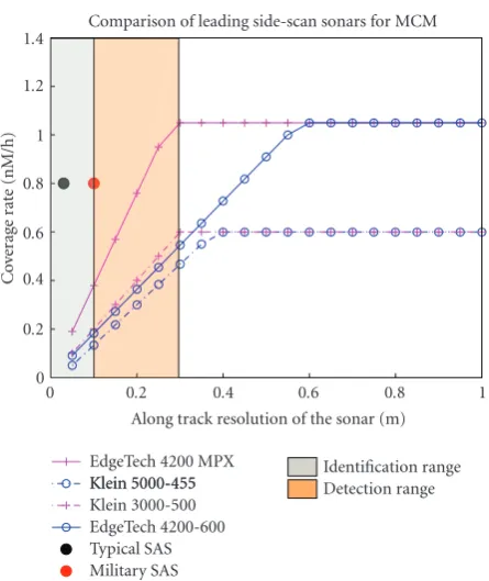
Figure 9: Ability to detect and identify targets as a function of resolution and coverage rate (Nm/h: nautical mile per hour) for the best sidescan and synthetic aperture sonars. The SAS sonars here are a typical 100–300 kHz sonar in optimal conditions for synthetic aperture.
models the anisotropic erosion of the rock due to underwater currents
Ffx,fy
= 1 α·f2
x + fy2
β, (2)
(d) Cluttered Environment. The cluttered environment is characterized by a random distribution of small rocks. A poisson distribution has been chosen for the spatial distribution of the rocks on the seabed as the mean number of occurrences is relatively small.
2.2. Targets. A separate module is provided for adding targets
into the environment.Figure 4displays the 3D models of 6
different targets. Location, size and material composition can
be adjusted by the user. The resulting sidescan images offer a
large data base for detection and classification algorithms. Nonmine targets can also be generated by varying parameters in this module. Several are used to test the
algorithms with results presented inSection 4.1.2.
2.3. The Sonar Image Generator. The sonar module computes the sidescan image from a given 3D environment. The simulator is ray-tracing-based and solves the sonar equation
[36] (given in (3)). Because (3) is an energetic equation,
phenomena such as multipaths are not taken into account.
For a monostatic sonar system, the sound propagation can be expressed from an energetic point of view as
XS=SL−2TL + TS + DI−NL−RL, (3)
where XS is the excess level, that is, the backscattering energy, SL is the Source Level of the projector, DI is the Directivity Index, TL is the Transmission Loss, NL is the Noise Level, RL is the Reverberation Level and TS is the Target Strength. All the parameters are measured in decibels (dB) relative to the
standard reference intensity of a 1μPa plane wave.
In a wide range of cases, a good approximation to transmission loss TL can be made by considering the process as a combination of free field spherical spreading and an added absorption loss. This working rule can be expressed as
TL=20 logr+αr, (4)
where r is the transmission range and αis an attenuation
coefficient expressed in dB/m. The attenuation coefficient
can be expressed as the sum of two chemical relaxation pro-cesses and the absorption of pure water. It can be computed
numerically thanks to the Francois-Garrison formula [37].
Reverberation Level is an important restricting factor in the detection process, especially in the context of MCM. At
short ranges, it represents the most significantnoise factor.
The surface reverberation can be developed as drawn in Figure 5, wheredAdefines the elementary surface subtended
by horizontal angledφand is dependent on the pulse length
τ and range. Returns from the front and rear ends of the
pulse determine the size of the elementary surface element,
dA. So, for the seabed contribution to reverberation level, we
can write
RL=SL−2TL +Ss+ 10 logcτ
2φr, (5)
where d is the altitude of the sonar, r is the range to the
seabed along the main axis of the transducer beam andtis
time.
Three types of seabed have been implemented: Rough Rock, Sandy Gravel and Very Fine Sand. A theoretical Bottom
Scattering Strength (Ss in (5)) can be computed thanks to
[30].
The source level SL is the power of the transmitter. It is a constant and given by the sonar manufacturer. For sidescan the SL is typically between 200 and 230 dB.
The Directivity Index (DI) is a sonar-dependent factor associated with directionality of the transducer system. The simulator includes a simple beam pattern derived from a continuous line array model of length l. The beam pattern function can be computed thanks to the following:
B(θ)=
sin(πl/λ) sinθ (πl/λ) sinθ
. (6)
Also any transducer beam pattern can be integrated into the simulator.
3 2 1 0
(M
et
ers)
0 1 2 3
(Meters) (a)
3 2 1 0
(M
et
ers)
0 1 2 3
(Meters) (b)
3 2 1 0
(M
et
ers)
0 1 2 3
(Meters) (c)
3 2 1 0
(M
et
ers)
0 1 2 3
(Meters) (d)
Figure10: Snapshot of the four targets. (a) Manta, on sand ripples, (b) Rockan on cluttered environment, (c) Cuboid on flat seabed, (d) Cylinder on sand ripples. The pixel size in these targets images is 5 cm.
using a Lambertian model. The reflectance factor in the Lambertian law is associated to the acoustic impedance. The simulator takes into account the acoustic impedance of the
target given by Z = ρ·cl, whereρ is the density of the
material, andclthe longitudinal sound speed in the material.
The sidescan simulator is designed for validity in the range of frequencies from 80 kHz to 300 kHz. We only consider one contribution for the ambient Noise Level: the thermal noise. For thermal agitation, the equivalent noise
spectrum level is given by the empirical formula [36]:
NL= −15 + 20 log f with f in kHz. (7)
The trajectory of the sonar platform is tuneable (as
shown inFigure 6). This allows multiview sidescan images
of the same environment.Figure 7displays sonar images of
the same scene with two different angles of view.
Further examples of typical images obtained for the
various types of seabed are shown inFigure 8.
3. Classifier
3.1. Target Recognition Using Sonar Images. Target recogni-tion in sonar imagery is a long-standing problem which has
attracted considerable attention [7–15]. However, the
reso-lution of the sensors available has limited not only the spec-trum of techniques applicable, but also their performances.
Most techniques for detection rely on matched filtering [38]
or statistical modeling [11,14], whilst recognition is mainly
model-based [10,13,15].
The limitations of current sidescan technology are
high-lighted inFigure 9. It would seem from this figure that only
0 10 20 30 40 50 60 70
M
isidentification
(%)
5 10 15 20 25 30
Pixel resolution (cm) Manta
Rockan
Cylinder Cube
Figure11: Misidentification of the four targets as a function of the pixel resolution. This is considering the highlight of the targets.
resolution needed for identification. However the boundaries drawn between detection and identification are more the results of general wisdom than solid scientific evidences.
New high resolution sonars such as SAS produce images which get closer to traditional optical imagery. This is also opening a new era of algorithm development for acoustics, as techniques recently developed in computer vision become more applicable. For example, the SAS system developed by NURC (MUSCLE) can achieve a 5 to 3 cm pixel resolution, almost independent of range. Thanks to this resolution, direct analysis of the target echo rather than traditional techniques based on its shadow become possible.
Identifying the resolution required to perform target classification is not a simple problem. In sonar, this has been
attempted by various authors [39–42], generally looking at
the minimum resolution required to distinguish a sphere from a cube and using information theory approaches. These techniques provide a lower bound on the minimum resolution required but tend to be over optimistic. We focus here on modern subspace algorithms based on PCA (Principal Component Analysis) as a mechanism to analyze the resolution needs for classification. Why focus on such techniques? The main reason is that they are very versatile and have been applied successfully to a variety of classical target identification problems. This has been demonstrated
recently on face recognition [43] and land-based object
detection problems [44].
3.2. Principal Component Analysis. The algorithm used in this paper for classification is based on the eigenfaces algorithm. The PCA-basedd eigenfaces approach has been
used for face recognition purposes [45,46] and is still close
to the state of the art for this application [43].
Assuming the training set is composed ofkimages of a
target. Each target imageMiis ann×mmatrix. TheMiare
converted into vectorsMiof dimension 1×n·m. A mean
image of the target is computed using the following:
Mmean= 1 k
k
i=1
Mi. (8)
The training vectors Mi are centered and normalized
according to (9). In the training set, the target is selected
from various ranges (from 5 m to 50 m from the sonar). The contrast and illumination change drastically through the training set. The normalization by the standard deviation
of the image reduce this effect. Let stdMi be the standard
deviation ofMi
Ti= Mi−Mmean stdMi
. (9)
Let T = [Ti] be the preprocessing training set of
dimensionk×n·m. The covariance matrixΩ =T·TT is
calculated. Theplargest eigenvalues ofΩare computed, and
the p corresponding eigenvectors form the decomposition
base of the target. The subspace Θtarget formed by the p
eigenvectors is called target space. The number of eigenvalues
phas been set to 20.
The classifier projects the test target image In to each
target space. We denotePΘtarget(In) the projection ofInin the
target space Θtarget. The estimated target targ is the target
corresponding to the minimum distance between In and
PΘtarget(In) as expressed in
targ=min
target
In−PΘtarget(In)
. (10)
PΘtarget(In) with the minimum distance represents the most compact space which represents the object under in-spection.
4. Results
In previous works [15, 16, 47, 48], target classification
algorithms using standard sidescan sonars have mainly been based on the analysis of the targets’ shadows. With high resolution sonars, we note that more information should be exploitable from the target’s highlight. In this section, we investigate the resolution needed for the PCA image-based classifier described earlier to classify using only the information carried by the highlight.
The sidescan simulator presented inSection 2will
pro-vide synthetic data in order to train and to test the PCA image-based classifier. All the sidescan images are generated with a randomly selected seafloor (from flat seabed, ripples and cluster environment), random sonar altitude (from 2 to 10 metres altitude) and random range for the targets (from 5 to 50 metres range).
For each experiment, two separate sets of sonar images have been computed, one specifically for training (in order
to compute the target spaceΘtarget) and one specifically for
1.2 1 0.8 0.6 0.4 0.2
(M
et
ers)
0.2 0.4 0.6 0.8 1 1.2 (Meters) Manta
(a)
1.2 1 0.8 0.6 0.4 0.2
0.2 0.4 0.6 0.8 1 1.2 (Meters) Rockan
(b)
1.2 1 0.8 0.6 0.4 0.2
0.2 0.4 0.6 0.8 1 1.2 (Meters) Cylinder
(c)
1.2 1 0.8 0.6 0.4 0.2
(M
et
ers)
0.2 0.4 0.6 0.8 1 1.2 (Meters) Cuboid
(d)
1.2 1 0.8 0.6 0.4 0.2
0.2 0.4 0.6 0.8 1 1.2 (Meters) Big hemisphere
(e)
1.2 1 0.8 0.6 0.4 0.2
0.2 0.4 0.6 0.8 1 1.2 (Meters) Hemisphere
(f)
1.2 1 0.8 0.6 0.4 0.2
0.2 0.4 0.6 0.8 1 1.2 (Meters) Box
(g)
Figure12: Snapshot of the targets used for classification. On the first line, the minelike targets with the Manta, the Rockan and the cylinder. On the second line, the nonmine targets with the cube, the two hemispheres, and the box shape target. The pixel size in these targets images is 5 cm.
0 0.2 0.4 0.6 0.8 1
0.05 0.1 0.15 0.2 0.25 0.3
M
isidentification
(%)
Pixel resolution (m) Box
Cube Cylinder Hemisphere
Small hemisphere Manta
Rockan (a)
0 0.2 0.4 0.6 0.8 1
0.05 0.1 0.15 0.2 0.25 0.3
M
isclassification
(%)
Pixel resolution (m) Mine-like object
Non mine object
(b)
Figure14: Snapshot of the shadow of the four targets (from left to
right: Manta, Rockan, Cube and Cylinder) to classify with different
orientations and backgrounds. The pixel size is these target images
is 5 cm. The size of each snapshot is 1.25 m×2.75 m.
0 10 20 30 40 50
0.05 0.1 0.15 0.2 0.25 0.3
M
isidentification
(%)
Pixel resolution (cm) Manta
Rockan
Cylinder Cube
Figure15: Percentage of misidentification versus the pixel resolu-tion for various target types. This considers the shadow of the target and not its echo.
and with a randomly selected seafloor have been used for training. A larger set of 40000 synthetic target images are used to test the classifier. The classifier is trained and tested
according to the algorithm described inSection 3.2.
4.1. What Precision Is Needed?
4.1.1. Identification. In this first experiment the PCA clas-sifier is train for identification. Assuming a minelike object has been detected and classified as a mine, the algorithm identifies the kind of mine the target Four targets have been chosen: a Manta mine (truncated cone with dimensions 98 cm lower diameter; 49 cm upper diameter; 47 cm height),
a Rockan mine (L × W ×H: 100 cm ×50 cm × 40 cm),
a cuboid with dimensions 100 cm×30 cm ×30 cm and a
cylinder 100 cm long and 30 cm in diameter.
Figure 10displays snapshots of the four different targets for a 5 cm sonar resolution.
The pixel resolution is tunable in the simulator. Sidescan simulation/classification processes have been run for 15
different pixel resolutions from 3 cm (high resolution sonar)
to 30 cm (low resolution sonar) covering the detection and
classification range of side looking sonars.Figure 11displays
the misidentification % of the four targets against the pixel resolution.
As expected, the image-based classifier fails at low resolu-tions. Between 15 and 20 cm resolution, which corresponds to the majority of standard sonar systems, classification based on the highlights is poor (between 50% and 80% correct classification). The results stabilize at around 5 cm resolution to reach around 95% correct classification.
In previous work involving face recognition where it has been shown that PCA techniques are not very robust
to rotation [49]. The algorithm can be optimized using
multiple subspaces for each nonsymmetric target, each of the subspaces covering a limited angular range.
4.1.2. Classification. In this section we extend the PCA classifier for underwater object classification purposes. A larger set of seven targets have been chosen with three minelike objects: the Manta, the Rockan, a cylinder 100 cm long and 30 cm diameter and four nonmine objects: a cuboid
with dimension 100 cm×50 cm×40 cm, two hemispheres
with diameters, respectively, 100 cm and 50 cm and a box
with dimension 70 cm × 70 cm × 40 cm. Note that the
nonmine targets have been chosen such as the dimension of the big hemisphere matches with the dimension of the Manta, and the dimension of the box matches with the
dimension of the Rockan. Figure 12provides snapshots of
the different targets.
As described inSection 4.1.1, two data sets for training
and testing have been produced. The target classification relies on two steps: at first the target is identify following
the same process asSection 4.1.1and then classified into two
classesminelikeandnonmine
Figure 13(a)displays the results of the identification step. the curves of misidentification for each target follow the
general pattern described earlier inSection 4.1.1with a low
misidentification (below 5%) for a pixel resolution lower
than 5 cm. In Figure 13(b), the results of the classification
between minelike andnonmineis showed. Contrary to the
identification process, the classification curves stabilise at higher pixel resolution (around 10 cm) to 2-3% misclassifi-cation.
In these examples we show that the identification task needs a higher pixel resolution that the classification task to match the same performances 95% correct identifica-tion/classification.
4.2. Identification with Shadow. As mentioned earlier, cur-rent sidescan ATR algorithms depend strongly on the target shadow for detection and classification. The usual
assumption made is:at low resolution the information relative
to the target is mostly contained in its shadow. In this section we aim to confirm this statement by using the classifier
We study here the quantity of information contained into the shape of the shadow, and how this information is retrievable depending on the pixel resolution.
Shadows are the result of the directional acoustic illumi-nation of a 3D target. They are therefore range dependent. For the purposes of this experiment, in order to remove the
effect of the range dependence of the shadows, the targets
are positioned at a fixed range of 25 m from the sensor. Image segments containing the target shadows are extracted
from the data.Figure 14displays snapshots of target shadows
with different orientations and backgrounds for a 5 cm pixel
resolution. We process the target shadow images in exactly in the same way as we did for the target highlight images in the previous sections. For each sonar resolution, 80 target shadows per object are used for training the classifier, and a set of 40000 shadow images is used for testing.
In total 15 training/classification simulations have been done for 15 sonar pixel resolutions (from 5 cm to 30 cm). Figure 15shows the percentage of misclassification versus the pixel resolution for various target types.
Concerning the Cylinder and Cuboid targets, their
shad-ows are very similar due the similar geometry. InFigure 14
it is almost impossible to distinguish visually between the two objects looking only at their shadows. In broadside for example, the two shadows have exactly the same rectangular shape, explaining why the confusion between these two objects is high.
For the Manta and Rockan targets, the misidentification curves stabilize near 0% misidentification below 20 cm sonar resolution. Therefore, for standard sidescan systems with a resolution in the 10–30 cm range, the target information can be extracted from the shadow with an excellent probability of correct identification. In comparison, correct identification using the target highlights at 20 cm resolution is about 50% (cf.Figure 11)
5. Conclusions and Future Work
In this paper, a new real-time realistic sidescan simulator has been presented. Thanks to the flexibility of this numerical
tool, realistic synthetic data can be generated at different pixel
resolutions. A subspace target identification technique based on PCA has been developed and used to evaluate the ability of modern sonar systems to identify a variety of targets.
The results processing shadow images back up the widely accepted idea that identification from current sonars at 10–20 cm resolution is reaching its performance limit. The advent of much higher resolution sonars has now made it possible to bring in and apply techniques new to the field from optical image processing. The PCA analyses presented here, operating on highlight as opposed solely to shadow, show that these can give a significant improvement in target identification and classification performance opening the
way for reinvigorated effort in this area.
The emergence of very high resolution sonar systems such as SAS and acoustic cameras will enable more advanced target identification techniques to be used very soon. The next phase of this work will be to validate and confirm these
using real SAS data. We are currently undertaking this phase in collaboration with the NATO Undersea Research Centre and DSTL under the UK Defense Research Centre program.
Acknowledgments
This work was supported by EPSRC and DSTL under
research contracts EP/H012354/1 and EP/F068956/1. The
authors also acknowledge support from the Scottish Funding Council for the Joint Research Institute in Signal and Image Processing between the University of Edinburgh and Heriot-Watt University which is a part of the Edinburgh Research Partnership in Engineering and Mathematics (ERPem).
References
[1] A. Bellettini, “Design and experimental results of a 300-kHz synthetic aperture sonar optimized for shallow-water
operations,”IEEE Journal of Oceanic Engineering, vol. 34, no.
3, pp. 285–293, 2009.
[2] B. G. Ferguson and R. J. Wyber, “Generalized framework for real aperture, synthetic aperture, and tomographic sonar
imaging,”IEEE Journal of Oceanic Engineering, vol. 34, no. 3,
pp. 225–238, 2009.
[3] E. O. Belcher, D. C. Lynn, H. Q. Dinh, and T. J. Laughlin, “Beamforming and imaging with acoustic lenses in small,
high-frequency sonars,” inProceedings of the Oceans
Confer-ence, pp. 1495–1499, September 1999.
[4] A. Goldman and I. Cohen, “Anomaly subspace detection
based on a multi-scale Markov random field model,”Signal
Processing, vol. 85, no. 3, pp. 463–479, 2005.
[5] F. Maussang, J. Chanussot, A. H´etet, and M. Amate, “Higher-order statistics for the detection of small objects in a noisy
background application on sonar imaging,”EURASIP Journal
on Advances in Signal Processing, vol. 2007, Article ID 47039, 17 pages, 2007.
[6] B. R. Calder, L. M. Linnett, and D. R. Carmichael, “Spatial
stochastic models for seabed object detection,” inDetection
and Remediation Technologies for Mines and Minelike Targets
II, Proceeding of SPIE, pp. 172–182, April 1997.
[7] M. Mignotte, C. Collet, P. Perez, and P. Bouthemy, “Hybrid genetic optimization and statistical model-based approach for
the classification of shadow shapes in sonar imagery,”IEEE
Transactions on Pattern Analysis and Machine Intelligence, vol. 22, no. 2, pp. 129–141, 2000.
[8] B. Calder, Bayesian spatial models for sonar image
interpre-tation, Ph.D. dissertation, Heriot-Watt University, September 1997.
[9] G. J. Dobeck, J. C. Hyland, and LE. D. Smedley, “Automated detection and classification of sea mines in sonar imagery,” in
Detection and Remediation Technologies for Mines and Minelike Targets II, Proceedings of SPIE, pp. 90–110, April 1997. [10] I. Quidu, J. PH. Malkasse, G. Burel, and P. Vilbe, “Mine
classification based on raw sonar data: an approach combining Fourier descriptors, statistical models and genetic algorithms,” inProceedings of the Oceans Conference, pp. 285–290, Septem-ber 2000.
[11] B. R. Calder, L. M. Linnett, and D. R. Carmichael, “Bayesian
approach to object detection in sidescan sonar,”IEE
[12] R. Balasubramanian and M. Stevenson, “Pattern
recogni-tion for underwater mine detecrecogni-tion,” in Proceedings of the
Computer-Aided Classification/Computer-Aided Design
Confer-ence, Halifax, Canada, November 2001.
[13] S. Reed, Y. Petillot, and J. Bell, “Automated approach to classification of mine-like objects in sidescan sonar using
highlight and shadow information,”IEE Proceedings: Radar,
Sonar and Navigation, vol. 151, no. 1, pp. 48–56, 2004. [14] S. Reed, Y. Petillot, and J. Bell, “Model-based approach to
the detection and classification of mines in sidescan sonar,”
Applied Optics, vol. 43, no. 2, pp. 237–246, 2004.
[15] E. Dura, J. Bell, and D. Lane, “Superellipse fitting for the recovery and classification of mine-like shapes in sidescan
sonar images,”IEEE Journal of Oceanic Engineering, vol. 33,
no. 4, pp. 434–444, 2008.
[16] B. Zerr, E. Bovio, and B. Stage, “Automatic mine classi-fication approach based on auv manoeuverability and the
cots side scan sonar,” in Proceedings of the Autonomous
Underwater Vehicle and Ocean Modelling Networks Conference (GOATS ’00), pp. 315–322, 2001.
[17] M. Azimi-Sadjadi, A. Jamshidi, and G. Dobeck, “Adaptive underwater target classification with multi-aspect decision
feedback,” inProceedings of the Computer-Aided Classification/
Computer-Aided Design Conference, Halifax, Canada, Novem-ber 2001.
[18] I. Quidu, J. PH. Malkasse, G. Burel, and P. Vilbe, “Mine
classification using a hybrid set of descriptors,” inProceedings
of the Oceans Conference, pp. 291–297, September 2000. [19] J. Fawcett, “Image-based classification of side-scan sonar
detections,” in Proceedings of the Computer-Aided
Classifi-cation/Computer-Aided Design Conference, Halifax, Canada, November 2001.
[20] S. Perry and L. Guan, “Detection of small man-made objects in multiple range sector scan imagery using neural networks,” inProceedings of the Computer-Aided Classification/Computer-Aided Design Conference, Halifax, Canada, November 2001. [21] C. Ciany and W. Zurawski, “Performance of computer aided
detection/computer aided classification and data fusion algorithms for automated detection and classification of
underwater mines,” in Proceedings of the Computer-Aided
Classification/Computer-Aided Design Conference, Halifax, Canada, November 2001.
[22] C. M. Ciany and J. Huang, “Computer aided detec-tion/computer aided classification and data fusion algorithms for automated detection and classification of underwater
mines,” inProceedings of the Oceans Conference, pp. 277–284,
September 2000.
[23] Y. Pailhas, C. Capus, K. Brown, and P. Moore, “Analysis and classification of broadband echoes using bio-inspired dolphin
pulses,”Journal of the Acoustical Society of America, vol. 127,
no. 6, pp. 3809–3820, 2010.
[24] C. Capus, Y. Pailhas, and K. Brown, “Classification of bottom-set targets from wideband echo responses to bio-inspired
sonar pulses,” inProceedings of the 4th International Conference
on Bio-acoustics, 2007.
[25] J. Bell, A model for the simulation of sidescan sonar, Ph.D.
dissertation, Heriot-Watt University, August 1995.
[26] A. J. Hunter, M. P. Hayes, and P. T. Gough, “Simulation of multiple-receiver, broadband interferometric SAS imagery,” in Proceeding of IEEE Oceans Conference, pp. 2629–2634, September 2003.
[27] J. M. Bell, “Application of optical ray tracing techniques to the
simulation of sonar images,”Optical Engineering, vol. 36, no.
6, pp. 1806–1813, 1997.
[28] G. R. Elston and J. M. Bell, “Pseudospectral time-domain modeling of non-Rayleigh reverberation: synthesis and
statis-tical analysis of a sidescan sonar image of sand ripples,”IEEE
Journal of Oceanic Engineering, vol. 29, no. 2, pp. 317–329, 2004.
[29] M. Pinto, “Design of synthetic aperture sonar systems for
high-resolution seabed imaging,” inProceedings of MTS/IEEE
Oceans Conference, Boston, Mass, USA, 2006.
[30] A. P. L. at the University of Washington, “High-Frequency Ocean Environmental Acoustic Models Handbook,” Tech. Rep. APLUW TR 9407, October 1994.
[31] B. Mandelbrot,The Fractal Geometry of Nature, W. H.
Free-man, 1982.
[32] A. P. Pentland, “Fractal-based description of natural scenes,”
IEEE Transactions on Pattern Analysis and Machine Intelligence, vol. 6, no. 6, pp. 661–674, 1984.
[33] R. F. Voss, Random Fractal Forgeries in Fundamental
Algo-rithms for Computer Graphics, R. A. Earnshaw, Ed., Springer, Berlin, Germany, 1985.
[34] P. A. Burrough, “Fractal dimensions of landscapes and other
environmental data,”Nature, vol. 294, no. 5838, pp. 240–242,
1981.
[35] S. Lovejoy, “Area-perimeter relation for rain and cloud areas,”
Science, vol. 216, no. 4542, pp. 185–187, 1982.
[36] R. J. Urick,Principles of Underwater Sound, McGraw-Hill, New
York, NY, USA, 3rd edition, 1975.
[37] R. E. Francois, “Sound absorption based on ocean measure-ments: Part I: pure water and magnesium sulfate
contribu-tions,”The Journal of the Acoustical Society of America, vol. 72,
no. 3, pp. 896–907, 1982.
[38] T. Aridgides, M. F. Fernandez, and G. J. Dobeck, “Adaptive three-dimensional range-crossrange-frequency filter process-ing strprocess-ing for sea mine classification in side scan sonar
imagery,” inDetection and Remediation Technologies for Mines
and Minelike Targets II, Proceedings of SPIE, pp. 111–122, April 1997.
[39] M. Pinto, “Performance index for shadow classification in
minehunting sonar,” in Proceedings of the UDT Conference,
1997.
[40] V. Myers and M. Pinto, “Bounding the performance of sidescan sonar automatic target recognition algorithms using
information theory,”IET Radar, Sonar and Navigation, vol. 1,
no. 4, pp. 266–273, 2007.
[41] R. T. Kessel, “Estimating the limitations that image resolution
and contrast place on target recognition,” inAutomatic Target
Recognition XII, Proceedings of SPIE, pp. 316–327, usa, April 2002.
[42] F. Florin, F. Van Zeebroeck, I. Quidu, and N. Le Bouffant,
“Classification performance of minehunting sonar: theory,
practical, results and operational applications,” inProceeedings
of the UDT Conference, 2003.
[43] J. Wright, A. Y. Yang, A. Ganesh, S. S. Sastry, and YI. Ma,
“Robust face recognition via sparse representation,” IEEE
Transactions on Pattern Analysis and Machine Intelligence, vol. 31, no. 2, pp. 210–227, 2009.
[44] A. Nayak, E. Trucco, A. Ahmad, and A. M. Wallace, “Sim-BIL: appearance-based simulation of burst-illumination laser
sequences,”IET Image Processing, vol. 2, no. 3, pp. 165–174,
2008.
[45] L. Sirovich and M. Kirby, “Low-dimensional procedure for the
characterization of human faces,”Journal of the Optical Society
[46] K. Etemad and R. Chellappa, “Discriminant analysis for
recognition of human face images,” Journal of the Optical
Society of America A, vol. 14, no. 8, pp. 1724–1733, 1997. [47] S. Reed, Y. Petillot, and J. Bell, “An automatic approach to the
detection and extraction of mine features in sidescan sonar,”
IEEE Journal of Oceanic Engineering, vol. 28, no. 1, pp. 90–105, 2003.
[48] V. L. Myers, “Image segmentation using iteration and fuzzy
logic,” in Proceedings of the Computer-Aided Classification/
Computer-Aided Design Conference, 2001.