Recent Advances in Explaining Hedge Fund
Returns: Implicit Factors and Exposures
Abstract
We survey articles covering how hedge funds returns are explained, using largely non-linear multifactor models that examine the non-non-linear pay-offs and exposures of hedge funds. We provide an integrated view of the implicit factor and statistical factor models that are largely able to explain the hedge fund return-generating process. We present their evolution through time by discussing pioneering studies that made a significant contribution to knowledge, and also recent innovative studies that examine hedge funds exposures using advanced econometric methods. This is the first review that analyzes very recent studies that explain a large part of hedge fund variation. We conclude by presenting some gaps for future research.
1 Introduction
A large and growing body of literature has investigated hedge fund performance
attribution through the use of implicit or statistical factor models (e.g. Billio,
Getmansky and Pelizzon, 2012; Akay, Senyuz, and Yoldas, 2013; O’Doherty, Savin,
and Tiwari, 2015). Investors want to know what is behind hedge fund return
variation and what to expect from different hedge fund strategies or funds with
different styles. Investors need to be familiar with the principles that enable them to
understand hedge fund performance behaviour. Although many studies describe the
role of factors or exposures of hedge funds in delivering excess returns to investors,
there is no survey that summarizes and discusses the results. This issue creates
confusion to investors who do not have a clear picture or a holistic interpretation of
the dynamics of hedge fund performance attribution.
The present study therefore closes an important gap. The aim of this study is to
survey the literature and investigate the hedge fund return generating process within
implicit or statistical factor models. This is the first survey and synthesis of older
literature to yield a historical perspective, along with a survey in more detail of
recent innovative studies that depict advances in hedge fund performance
attribution1. Hence readers will have an integrated view and a deeper understanding
of hedge funds. Our findings both make life easier for hedge fund investors and
highlight opportunities for further research.
Our main conclusions are that early studies (e.g. Sharpe, 1992), through the use of
asset categories or where the fund manager invests. They depicted a static
representation of hedge fund performance attribution. Then there was a development
toward non-linear models that tried to explain hedge funds’ performance as option
portfolios (e.g. Fung and Hsieh, 2004; Agarwal and Naik, 2004). Nevertheless, in
recent years there have been several studies (e.g. Patton and Ramadorai, 2013; Bali,
Brown and Caglayan, 2014; O’Doherty, Savin, and Tiwari, 2015) that use more
advanced models regarding hedge fund exposures. They confirmed previous studies
that hedge funds have non-linear returns in relation to the market return, but they
moved further and showed how these non-linear exposures change over time
according to financial conditions. Different strategies frequently have different
exposures. However, there are a few exposures that are valid for virtually every
hedge fund strategy (equity market, volatility, liquidity). Furthermore, systematic
risk and more specifically macroeconomic risk have a significant role in explaining
hedge fund performance for nearly all strategies. Higher moment factors provide
extra explanatory power to the models.
This paper makes a number of important contributions to the understanding of the
hedge fund literature. First, it covers a significant gap by presenting a survey that
summarizes and discusses studies examining hedge fund performance attribution
within statistical factors and exposures. It demonstrates a historical perspective by
combining earlier and more recent innovative studies, discussing their strengths and
weaknesses. Therefore the reader is able to look at the dynamic nature of the
literature explaining hedge fund returns. This study assist investors in their asset
allocation process in two ways: it facilitates a deeper understanding of what is
behind hedge fund return variation and it also enables investors to know what to
identified some gaps for future research. An example is the absence of a unified
framework that takes into consideration the comprehensive macroeconomic
environment along with the internal structure of the hedge fund industry in
explaining returns, or identifying the proportion of alpha affected by each of the
underlying factors.
We start off in section 2 with a review of extant hedge fund literature review papers.
In section 3 we depict different general approaches in measuring the performance of
all hedge fund strategies2. Section 4 briefly reviews earlier linear studies. Section 5
reviews in detail the most recent non-linear models within the bottom-up, up-bottom,
and alternative modeling approaches, as we describe later. In the final section 6 we
summarize the key conclusions and reveal some gaps that should be addressed in
future research.
2 Extant Hedge Fund Literature Review Papers
In this section we briefly discuss the extant hedge fund literature surveys. These
consist of two very recent and two earlier papers. They deal with different aspects of
hedge funds, including hedge fund performance attribution that we address
specifically in this paper. For brevity we do not review the papers covered in these
papers, as many of them are covered later in this paper and the reader can also refer
to these other review papers.
An interesting general study is from Getmansky, Lee, and Lo (2015) that replicated
implications for the efficient market hypothesis, financial regulation and systematic
risk among other areas. Getmansky et al. considered four perspectives on the hedge
fund industry: the investor’s perspective, the manager’s perspective, the regulator’s
perspective and the academic perspective. By reviewing several aspects of the hedge
fund literature and their implications for stakeholders in the hedge fund industry the
authors shone a light on two investors’ myths: first, that hedge funds comprise a
homogenous asset class that have similar investment characteristics and returns, and
second that all hedge funds are unique with no commonalities and, hence, no
implications for diversification or systematic risk.
Similar to the above is a survey from Agarwal, Mullally, and Naik (2015) in that it
examined several aspects of hedge funds such as hedge fund performance
(time-series and cross-sectional variation), the sources and nature of risks related to
managerial incentives and sources of capital, and the role of hedge funds in the
financial system. Concerning performance evaluation and attribution, the authors
suggested that the spectrum of risk factors explaining hedge funds variation is very
broad. The key challenge is the identification of a parsimonious set of factors with
greater availability of time-series data. This is because with more data we are more
likely to be able to eliminate spurious factors that do not stand the test of time.
Finally, the authors assert that there is substantial evidence that at least a subset of
hedge fund managers possess skill. Specifically there is evidence of managerial skill
in terms of their timing ability and their delayed disclosure of certain security
holdings.
An earlier study came from Fung and Hsieh (2006). They examined the growth of
CISDM databases using the framework from their 1997 paper. By putting forward a
simple model of how hedge funds do business they pulled together some of the
important issues involving investors in hedge fund products, financial intermediaries,
and regulators into a single framework. This framework revealed a fundamental
question regarding the identification of systematic risk factors inherent in hedge fund
strategies. In addition, the identification of these risk factors was the key input to
important questions such as optimal contrast design between buyers and sellers of
hedge fund products and explaining large changes in the hedge fund industry. In
their simple hedge fund business model the authors argued that apparent style
changes are consistent with fund managers maximizing their enterprise value, by
diversifying the impact of different life cycles of hedge fund strategies. Moreover the
pricing discovery process of a hedge fund firm favors those fund managers with a
steady, diversified stream of fee income. Thus this could reduce excessive risk taking
by individual fund managers.
Given that there is a concern over whether traditional metrics and tools for portfolio
measurement and risk management are applicable to hedge funds (e.g. due to serial
correlations in fund returns caused by illiquidity and smoothed returns), Lo (2005)
briefly reviewed and described hedge fund properties. He also developed new tools
and metrics when analyzing hedge funds. Using the CSFB/Tremont indices and the
TASS database and applying an econometric model using smoothed returns and
adjustments for the Sharpe ratio and other risk and return metrics, Lo showed that
serial correlation can have a significant impact on performance measures such as the
Sharpe ratio, with an overstatement of approximately 70 percent. He also addressed
hedge funds’ positive alphas come not only from seeking returns but also from adroit
risk management. Understanding the risk preferences of investors and fund managers
is an important element for proper risk management and investment policy.
In summary, four papers in the last decade conducted reviews of the academic
literature on hedge funds. They reached several valuable conclusions, however no
review paper has concentrated on how hedge fund returns have been explained. It is
this that we focus on in the rest of this paper, looking in particular at recent work on
non-linear models that had not been done at the time of the Lo (2005) and Fung and
Hsieh (2006) papers. However, we start in section 3 by describing different general
approaches towards hedge fund performance measurement.
3 Model Categories
In this section we present two general categories of models: absolute pricing models
and relative value models. Then we focus on two different statistical approaches:
Principal Component Analysis and Common Factor Analysis.
Generally speaking, asset pricing models are divided into two main categories: (i)
absolute pricing models and (ii) relative value models (Lhabitant, 2004 and 2007).
The first category consists of fundamental equilibrium models and
consumption-based models in combination with many macro-economic models. They use asset
pricing theory and price each asset individually taking into consideration its
exposures. They give an economic interpretation of why prices are what they are and
why exposures are what they are. In addition they are supposed to predict price
models explores the evidence of the different asset pricing rather than trying to fit an
explanation of the financial markets. They price each asset by taking into
consideration the prices of some other assets that are extraneous. In other words,
they provide a plain illustration of how the financial world works. A typical well
known example is the Black-Scholes (1973) formula that computes an option price
in regard to its underlying asset price, disregarding whether that asset is fairly priced
by the market. The factor models that we mention in this study belong to the
category of relative price models. They price or evaluate hedge funds in regard to the
market or any other risk factors. They do not concentrate on what induces the
primitive factors, the market or factor risk premium, or the risk exposures accepted
by the fund managers.
The majority of the factor (or relative price) models in this study use a two-stage
approach: At the beginning, they hypothesize that hedge funds returns are specific
functions of macro-economic and micro-economic factors (variables). Second, they
test those initial assumptions and assess the sensitivity of hedge funds returns to
those assumptions. Factor models determine the relationships between a large
number of variables (for instance fund returns) and describe these relationships in
terms of their common underlying dimensions, so called ‘factors’. Hence, there is the
advantage of dimensionality reduction because it sums up the information that is
contained in a large number of original values (hedge funds returns) into a smaller
set of factors with a minimum loss of information. In other words, via factor models
we simplify the covariance matrix (correlation or covariance among the returns of all
Amenc, Sfeir and Martellini (2002) report four types of factor models. These are: (1)
Explicit macro factors: These are macro-economic variables that are calculated
either as predictive variables or adopted ex-post to measure market sensitivities in
relation to some macroeconomic parameters. (2) Explicit index factor model: In these
models each factor is investable and represents some index or fund available as an
ETF (Exchange Trading Funds) or futures contract. (3) Explicit micro factor models:
These microeconomic parameters (or variables) that refer to fund-specific features
are estimated and forecast in a comparable manner as the explicit factor models. (4)
Implicit factor models: These implicit factors are mainly derived through Principal
Component Analysis (PCA) or Common Factor Analysis (CFA) and are regarded as
a merely statistical approach. An analogous classification is suggested by Connor
(1995) with the use of three types of factor models that are available for examining
asset returns, named as: Macroeconomic factor models, Fundamental factor models
and Statistical factor models.
In this part of our review we deal with statistical or implicit factor models.
Regarding those factor models there are two widely-used methodologies that are
used to distinguish the underlying factors: (i) Principal Component Analysis (PCA)
and (ii) Common Factor Analysis (CFA). We explain and analyse those two
methodologies and studies with regard to hedge funds.
3.1 Principal Components Analysis
The PCA methodology was first described by Pearson (1901). Implicit factors are
obtained via this approach. The purpose is to explain the return series of observed
factors are extracted from the time series of returns. In other words, the main
objective of PCA is to explain the behaviour of a number of correlated variables
using a smaller number of uncorrelated and unobserved implied variables or implicit
factors called principal components.
Fung and Hsieh (1997) used PCA to extract implicit factors in order to provide a
quantitative classification of hedge funds based on returns alone. They took into
consideration the location (market) as well the strategy (investment style) followed
by managers. The returns are supposed to be correlated to each other even though
they might not be linearly correlated to the returns of asset markets. They used a
database (1991-1995) from Paradigm LDC and from TASS Management. They
found that five principal components jointly accounted for 43% of the return
variance of hedge funds. They assigned concise names to these components: (1)
Trend-following strategies on diversified markets such as managed futures and
CTAs (Commodity Trading Advisors), (2) Global/macro funds, (3) Long/short
equity funds, (4) Funds with trend-following strategies specialized in major
currencies, (5) Distressed securities funds.
Later, Amenc, Martellini and Faff (2003) used PCA in creating a passive hedge fund
index or index of indices. Their method was a natural generalization of the equally
weighted portfolio of indices. Using PCA they created a portfolio of indices with
appropriate weights so that the combination of indices captured the largest possible
amount of information contained in the data (time-series returns) of those indices.
The first component was a candidate for a pure style index. This component caught a
index of indices is always more representative than any competing index upon which
it is based. Furthermore, an index of indices is consistently less biased than the
average of the set of indices it is derived from.
Additional authors who used PCA are Christiansen, Madsen and Christiansen (2003)
so as to identify the minimum number of components needed to describe the returns
of hedge funds from the CISDM database (1999-2002). They found that there were
five components, and by comparing these with the qualitative self-reported
classifications of hedge funds they identified five different strategies that could
explain greater than 60% of hedge fund return variation (Opportunistic/Sector, Event
Driven, Global Macro, Value and Market Neutral Arbitrage). It is evident from the
above papers that using four to five components is sufficient to explain a large part
of hedge fund returns.
3.2 Common Factor Analysis
The second statistical approach that is used more often in the literature is the
Common Factor Analysis (CFA). Its goal is identical to PCA, which is to transform a
number of correlated variables into a smaller number (dimensionality reduction) of
uncorrelated variables, that is, factors. Nevertheless, there is a great difference with
PCA. Here, the underlying factors are observable and clearly stated by the
researcher carrying out explanatory and/or confirmatory analysis. They are not just
implied by the data. As with PCA, the number of factors should be as small as
feasible in order to have the advantages of dimensionality reduction. However, the
researcher is making a trade-off between the dimensionality reduction and the
It is very common in factor analysis to choose factors on an ad hoc basis. The basic
principle is to pick up variables that are considered most probably to influence asset
returns. A researcher should take into consideration quantitative and qualitative
approaches in order to decide which factors to use. Furthermore, a researcher should
look for evidence from the empirical asset pricing literature. For many years
researchers looked for factors3 that explained and influenced the cross-sections of
expected returns.
Certain models that are extensions of the basic CAPM model have heavily
influenced hedge funds models. These are Fama and French (1993), using the size
and book to price ratio and Carhart (1997) that included the momentum as a fourth
factor. Other more recent models are Fung and Hsieh’s (2004) seven factor model, or
Capocci’s (2007) fourteen factor model. In the following two sections we present
some earlier and some more recent studies using implicit factor models that are
useful to reveal hedge funds exposures and explain their returns. A branch of the
CFA approach is the Asset-Based style (ABS), factors where the factors are
constructed by trading in the appropriate securities within the underlying
conventional assets (e.g. bonds or equities) that mimic the returns of hedge funds
(please see section 5.1).
Last but not least, one important application of factor models is hedge fund
replication. There is a distinction between traded factors (e.g. market and size
factors) and non-traded factors (e.g. volatility or liquidity), the latter of which are not
readily tradeable. Investors may therefore encounter problems in their replication. In
4 Linear Factor Models
In this section we briefly discuss some linear multi-factor models that are considered
to be key studies in the hedge fund literature4. It is known that linear multi-factors
models are based on the general linear equation model (Ross, 1976). In addition to
the market factor (Sharpe, 1964) the most popular is the Fama and French (1993)
model with the SMB (small minus large) and HML (high minus low book to market
ratio) factors. Carhart (1997) was the first who used the momentum factor
(Jegadeesh and Titman, 1993) as the fourth factor – a zero investment portfolio that
is long in past winners and short in past losers. His model is an extension of the
Fama and French factor model. All these previous factors are extensively used in the
hedge fund academic literature.
We first consider style analysis-trading factors so as to introduce the reader gently to
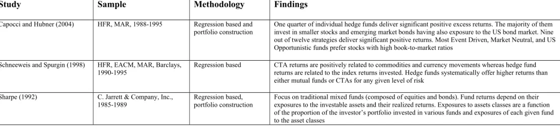
further linear and non-linear models. Therefore, we start from Sharpe (1992). Sharpe
used an asset class factor model implementing style analysis as a substantial
complement to other methodologies designed to assist investors achieve their targets
in a cost-effective manner. He used a model composed of twelve asset classes to
analyse the performance of funds between 1985 and 1989. The twelve asset classes
were: (1) T-bills, (2) Intermediate-term Govt. Bonds, (3) Long-term Govt. Bonds,
(4) Corporate Bonds, (5) Mortgage-Related Securities, (6) Large Cap Value Stocks,
(7) Large Cap Growth Stocks, (8) Medium Cap Stocks, (9) Small Cap Stocks (10)
Non-U.S. Bonds, (11) European Stocks and (12) Japanese Stocks. The variation of
fund returns in any specific period could be associated with the combined effects of
their exposures to these asset classes and the realized returns on these classes. Those
investor’s portfolio invested in the various funds and second the exposures of each
given fund to the asset classes. The exposures of a fund to wider asset classes
depended on two elements: the amount of money that the fund had invested in
various securities and the exposures of the securities to the asset class.
Sharpe’s (1992) style analysis can be used to appraise the behaviour of a fund
manager’s exposures to asset classes over a specific time period. Moreover it can be
used to measure a fund manager’s relative performance, in other words the value
added by her skills (alpha). A passive hedge fund manager provides investors with
an investment style whereas an active hedge fund manager provides both style and
selection. Thus we can determine the terms of active and passive management. An
investor may choose a set of asset classes that is superior to the performance of the
‘standard’ static mix and fulfils the requirement for higher fees. As a result, fund
selection return according to Sharpe (1992) is denoted as the difference between the
fund’s return and that of a passive mix with the same style. Once the styles of an
investor’s funds have been estimated it is possible to estimate the effective asset mix.
The effective asset mix reflects the style of the investor’s overall portfolio.
The model for explaining the results of traditional mixed funds (composed of
equities and bonds) first introduced by Sharpe (1992) is limited to funds that pursue
a long- only strategy. However, hedge funds are much more flexible and can also use
short selling and leveraging. These trading strategies of hedge funds lead to
option-like structures that are not covered by the basic Sharpe model or other similar
models. Confronting that problem, Fung and Hsieh’s (1997) study is presented in
Schneeweis and Spurgin (1998) used factors designed to capture the trading
opportunities available to CTAs or hedge funds as a means of forecasting return
performance. They used the databases of HFR, EACM, MAR and Barclays from
1990 to 1995. They considered the following factors to examine the returns to active
management of hedge funds, CTAs and mutual funds: (1) a natural return to owning
financial and real assets, (2) the use of both short and long positions, (3) the
exploitation of the indices’ intermonth volatility and (4) the exploitation of market
inefficiencies that result in temporary trends in prices. These factors were able to
significantly explain the differences in investment returns within each investment
grouping. Using multivariate regressions they showed that CTA returns are
positively related to commodity market trends. Hedge funds were related to the
returns of the index which they were investing, whereas they offer higher returns
than CTAs for any given level of risk.
A few years later, Capocci and Hubner (2004) examined hedge funds’ behaviour
from 1984 to 2000 (HFR, MAR) using various asset pricing models. Those included
an extended form of Carhart’s (1997) model, combined with the Fama and French
(1998) and Agarwal and Naik (2000) models plus one more factor that takes into
consideration the fact that hedge funds may invest in Emerging Markets. According
to the authors, that combined model better explained variations of hedge funds over
time than other studies, especially for Event Driven, U.S Opportunities, Global
Macro, Equity non-hedge and Sector Funds. The performance analysis showed that
one quarter of individual hedge funds delivered significant positive excess returns.
The majority of them preferred to invest in smaller stocks and also invest in
returns. Most Event Driven, Market Neutral and US Opportunistic funds prefer
stocks with high book-to-market ratios.
To sum up, there are several studies (e.g. Sharpe, 1992; Capocci and Hubner, 2004)
that examined hedge fund performance under a linear framework. However, linear
models are more suitable for traditional mixed funds (investing in equity and bonds).
Moreover they cannot capture the time variation of funds’ exposures. Some of these
issues are addressed by the non-linear factor models that are presented in the
following section5.
5 Non Linear Factor Models
Beyond the linear factor models that were used for explaining hedge fund returns
during the earlier years there is a development toward non-linear models. These try
to capture the exposures and the non-linear payoffs of hedge fund returns in relation
to their risk or market returns6. In general, there are two different approaches:
bottom-up (or indirect) and up-bottom (or direct). The former starts with the
underlying assets (e.g. stocks or bonds) to find the sources of hedge funds’ returns. It
involves replicating hedge fund portfolios by trading in the correspondent securities.
These trading constructed factors are defined as asset-based style (ABS) factors
(Fund and Hsieh, 2002a). The latter approach starts with identifying the sources of
hedge fund returns and relates pre-specified risk factors for hedge fund performance
attribution. It uses additional factors that better explain hedge fund returns. We also
present a third approach (an extension of the up-bottom) that deals with
5.1 Bottom-Up Approach
Option Portfolios and Trend Followers
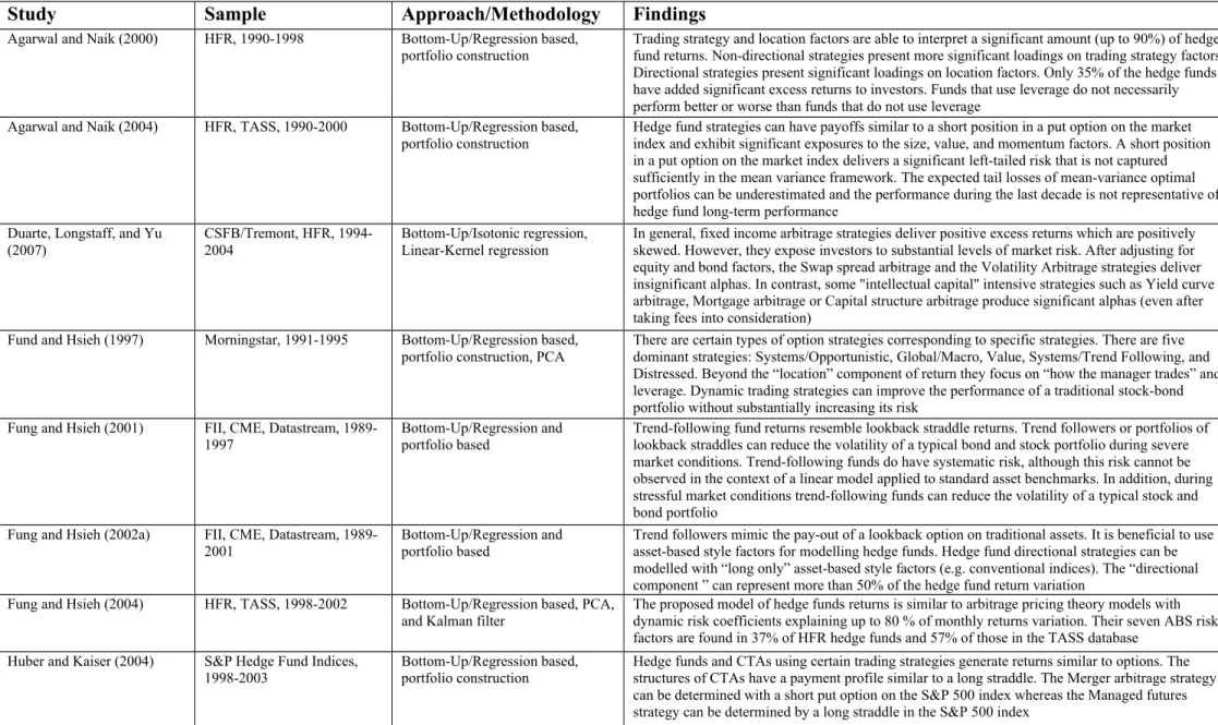
In this sub-section, we begin with Fung and Hsieh (1997) who provided a useful
characterization of the type of option strategy that one should expect when analysing
hedge fund returns. Then we proceed with the Fung and Hsieh (2001) study which
showed how to model hedge funds returns by concentrating on the ‘trend-following’
strategy. Examining futures and option futures, they demonstrated empirically that
the returns of trend-following funds resemble lookback straddle returns8. Fung and
Hsieh (2002a) extended their 2001 study to construct asset-based style factors. They
demonstrated a model that could predict the returns behaviour of trend following
strategies during certain market conditions. Fung and Hsieh (2004) was another
extension of their previous work in 2001 and 2002a on asset-based style (ABS)
factors. It proposed a model of hedge funds returns that is comparable to models
depending on arbitrage pricing theory with dynamic risk coefficients. Huber and
Kaiser (2004) confirmed Fung and Hsieh (1997, 2001) that CTAs have a payoff
profile similar to a long straddle9.
The authors Fung and Hsieh (1997) raised the issue of considering hedge funds as
option portfolios. Their study is an extension of Sharpe’s (1992) style analysis as
beyond the “location” component or factor of returns (which tell us the asset
categories or where the manager trades using a static buy and hold policy) they
added two other components: ‘Trading strategy factors’ (the way the manager trades,
denoting the type of dynamic strategy) and the ‘leverage factor’ (a scaling factor, the
quantify their statement (modelling hedge funds as option portfolios) and identify the
location and trading strategy factors, the authors used a relatively simple method that
is equivalent to non-parametric regression. They compared the performance returns
of hedge funds strategies versus U.S. equities (S&P 500) in five different economic
conditions (from worst to best). As suspected the short-only strategy had no
option-like feature and behaved almost exactly the opposite of equities. The CTA strategy
had a return profile close to a straddle on equities. The global macro strategy
performed like a short put on the S&P 500 and had an approximately linear profile
with regard to the USD/JPY exchange rate. Finally, the distressed securities and risk
arbitrage strategies also behaved like short puts on the S&P 500. Ultimately, Fung
and Hsieh (1997) provided a convenient characterization of the type of option
strategy that one should anticipate when dealing with funds’ returns, as hedge fund
strategies are highly dynamic (e.g. using derivatives, short-selling etc.). Moreover,
their study showed that there are five dominant strategies10 in hedge funds having
lower correlations with standard asset returns and mutual fund returns.
A few years later, Fung and Hsieh (2001) showed a way to model hedge funds
returns by concentrating on the well-known ‘trend-following’ strategy. They
examined futures and option futures from the Futures Industry Institute (FII), The
Chicago Mercantile Exchange (CME) and Datastream. They used a general
methodology for understanding hedge fund risk by modeling a specific trading
strategy which is widely referred as “trend following” within the industry. They
demonstrated empirically that the returns of trend-following funds resemble
lookback straddle returns. They explored hedge funds returns through modelling the
Given the market prices in any specific time period, the optimal pay-out of any
trend-following strategy should be equal to the one that bought at the lowest price
and sold at the highest price. It was for this reason that Fung and Hsieh (2001)
suggested using a lookback straddle. Indeed, the lookback straddle is of specific
interest due to its close connection to the return profiles of trend-following hedge
funds. The majority of CTAs or managed futures funds are in fact ‘trend-followers’
(or primitive trading strategies). The payoff of a perfect market timer who may take
long only positions should be very similar to the payoff from holding a call option.
However, if the flawless market timer may take long or short positions, this would
correspond to a perfect trend follower who could ‘buy low and sell high’. This is
equivalent to the payoff of a lookback straddle. Therefore, the lookback straddle can
be regarded as a primitive trading strategy exploited by market timers.
Fung and Hsieh (2001) showed that a lookback straddle is better fitted to capture the
principle of trend following strategies than simple standard asset benchmarks.
Trend-following funds have a systematic risk that cannot be captured by linear-factor
models applied to standard asset benchmarks. Also, trend-followers or portfolios of
lookback straddles can reduce the volatility of a typical bond and stock portfolio
during severe market downturns. However, it is important to mention that it is not
possible to have a unique benchmark that can be used to model the performance of
every trend follower. That is because there are significant dissimilarities in trading
strategies among trend-following funds.
Extending their 2001 study, Fung and Hsieh (2002a) used previously-developed
models to build asset-based style factors. They demonstrated a model that can
particularly during stressful market conditions such as those of September 2001. In
this study the authors added almost four years of data (1998 to 2001) since their
publication of 2001. Hence, they provided out-of-sample validation for their finding
that trend followers have returns characteristics that mimic the payout of a lookback
option on traditional assets. They showed that it is beneficial to model hedge funds
strategies using asset-based style factors. Hedge fund directional strategies can be
modelled with “long only” asset-based style factors and the “directional component”
represents more than 50 percent of the hedge fund return variation.
Fung and Hsieh’s 2004 study was an extension of their previous 2001 and 2002
papers on asset-based style (ABS) factors. It proposed a model of hedge fund returns
that is comparable to models based on arbitrage pricing theory, with dynamic risk
coefficients. They examined data from HFR and TASS databases for 1998 to 2002
and identified seven ABS factors to create hedge fund benchmarks that capture
hedge funds’ common risk factors. The seven ABS factors were two equity factors
(market and size), two fixed income factors (change in bond yield and change in
credit spread yield), and three trend-following factors (lookback straddles on bonds,
commodities, and currencies). Using funds of funds as a proxy for hedge fund
portfolios these factors were able to explain up to 80 percent (as represented by the
R-squares and depending on which time period they used) of monthly return
variations. Regarding the average hedge fund portfolio (using as proxy the HFR fund
of funds index), they found that it had systematic exposures to directional equity and
interest rates odds (bets), but they also had exposures to long equity and credit
events. The authors also used the Kalman Filtering technique with a set of exogenous
The final paper that we cover in this section on non-linear models is Huber and
Kaiser (2004). They supported Fung and Hsieh (1997, 2001) in that, because hedge
funds trade in a flexible way, their strategies lead to option-like structures that cannot
be covered by the classic Sharpe model. They explained how these option-like
structures come about. Thus hedge funds and CTAs using certain trading strategies
generate returns similar to options. In particular, the structures of CTAs have a
payoff profile similar to a long straddle. In their research, the authors presented an
investigation of the risk factors affecting the nine Standard & Poor’s Hedge Fund
Indices. Daily data about hedge funds indices were available from 1998 to 2003. The
highest return was achieved by the Equity Long/Short basket (23.6% p.a.) followed
by Convertible Arbitrage (21.8%) and Managed Futures (19.2%). The poorest
performers were Fixed Income Arbitrage (3.9%) and Merger Arbitrage (6.9%). The
authors used the classical Sharpe model equation using several factors Fk. The
empirical section of their study explained the risk factors of the Standard & Poor’s
Hedge Fund Indices taking the option-like futures into account. For instance merger
arbitrage had a significant determinant similar to a short put on the S&P index, and
managed futures, a long straddle on the S&P 500 index.
Option-Based Buy and Hold Strategies
In this sub-section we present the other line of research originating from Agarwal
and Naik (2000), who suggested a general asset factor model consisting of excess
returns on passive option-based strategies and on buy-and-hold strategies. In a later
study (2004) they focused on the systematic risk exposures of hedge funds that
practise buy-and-hold and option-based strategies. A more recent study that we
strategies, showing that “market neutral” strategies impose substantial risk exposures
on investors.
Agarwal and Naik (2000) suggested a general asset factor model consisting of excess
returns on passive option-based strategies and on buy-and-hold strategies. Despite
the fact that many hedge funds implement dynamic strategies, they found that a
small number of simple option writing/buying strategies were sufficient to explain a
large part of the variation in hedge fund returns over time. Using the Hedge Fund
Research Database from 1990 to 1998 (hedge fund indices), they evaluated the
performance of hedge funds that adopted different strategies (especially Event
Driven and Relative Value Arbitrage) using a general asset class factor model
composed of excess return on Location (buy-and-hold) and on Trading Strategy
(option writing/buying) factors.
Agarwal and Naik presented four main findings: First their model composed of
Trading Strategy factors and Location factors was able to interpret a significant
amount (up to 93%) of hedge funds’ returns over time. Second, non-directional
strategies displayed more significant loadings on Trading Strategy factors whereas
directional strategies displayed significant loadings on Location factors. They found
that in the early 1990s 38% of hedge funds added significant value (excess return or
alpha) compared to 28% of hedge funds that added value in the late 1990s. Last but
not least, leveraged funds did not consistently perform better or worse than funds
that did not use leverage.
HFR and TASS (hedge fund indices, 1990-2000). They found that a large number of
equity-oriented hedge funds strategies had payoffs similar to a short position in a put
option on the market index. This was in alignment with findings from other studies
such Awargal and Naik (2000) and Fund and Hsieh (1997) concerning the payoff
style of some hedge funds strategies. They found that a short position in a put option
on the market index brought a significant left-tail risk that was not captured
sufficiently in the mean-variance framework. Hence, they used a mean-conditional
value-at-risk framework and they demonstrated the degree to which the
mean-variance framework underestimated the tail risk, also showing that the last decade is
not representative of long term hedge fund performance.
In order to identify the linear and non-linear risks of a wide range of hedge funds
strategies they used buy-and-hold and option-based risk factors. They followed a
three-step approach: First they considered the loading coefficients (betas) using the
returns of standard asset classes and options on them as factors. Then they
constructed replicating portfolios that best explained the in-sample variation in hedge
funds returns. Finally they examined how well those replicating portfolios caught the
out-of sample performance of hedge funds. They conducted an analysis not only at
the index level, but also at the individual hedge fund level. As well as their
characterization of a non-linear relationship between portfolio return and its risk
when examining hedge funds, Agarwal and Naik (2004) found that hedge funds
exhibited significant exposures to Fama and French’s (1993) three-factor model and
Carhart’s (1997) momentum factor.
A more recent study using the ABS approach was from Duarte, Longstaff, and Yu
using the CSFB/Tremont and HFR databases from 1994-2004. Implementing
isotonic regression and linear-kernel regressions, they found all five strategies
exhibited positive excess returns. Some strategies such as yield curve arbitrage,
mortgage arbitrage and capital structure arbitrage presented significant positive
alphas (even after taking fees into consideration) as they required the most
“intellectual capital” to implement. They also found that, with the exception of the
volatility arbitrage strategy, the returns had positive skewness. Moreover, several so
called “market-neutral” arbitrage strategies imposed substantial risk exposures such
as equity and bond market factors on investors. However, they found little evidence
that these strategies exposed investors to substantial downside risk.
All the studies we have covered in this sub-section have been non-linear models that
tried to explain hedge funds’ performance as option portfolios. Fung and Hsieh
(1997) provided a useful characterization of the type of option strategy that one
should expect when analyzing hedge funds returns. Fung and Hsieh (2001, 2002)
repeatedly demonstrated empirically that returns of trend-following strategies
resemble lookback straddle returns. The same authors in 2004 presented the seven
factor model that was able to capture the common risk ABS factors in hedge funds.
Huber and Kaiser (2004) verified Fung and Hsieh (1997, 2001)’s results. They also
showed that hedge funds (especially those using a convergence strategy) also have
option-like return structures. Agarwal and Naik (2000 and 2004) suggested a factor
model based on passive option-based strategies and buy-and-hold strategies to
benchmark the performance of hedge funds. Their findings were consistent with
Fung and Hsieh (1997) concerning the payoff style of some hedge fund strategies.
were not so neutral for investors and some fixed income strategies required the most
“intellectual capital” to implement.
Although these studies are important to conceptually explain hedge funds returns
using non-linear models, we believe that there is a weakness as those perspectives
may not help investors in a practical way to choose and evaluate hedge funds. This is
because, first, these exposures are not static and change very often (see sub-section
5.3) and, second, these factors are not easy to replicate by an investor. Moreover,
some strategies (such as global macro or multi strategy) are not well defined hence
are difficult to replicate. We discuss this issue further in section 5.3.
5.2 Up-Bottom Approach
In this sub-section we deal with up-bottom approaches that in general use additional
factors that better explain hedge fund returns and also statistical techniques refining
these risk factors within the multi-factor models. Later studies, use more advanced
econometric techniques. We begin with two studies of Patton (2009) and Bali,
Brown, and Caglayan (2012) that have examined hedge funds’ claim of market
neutrality. Given the evidence that hedge funds contain systematic risk we proceed
further to studies that attribute hedge fund performance to various risks.
Market Neutrality
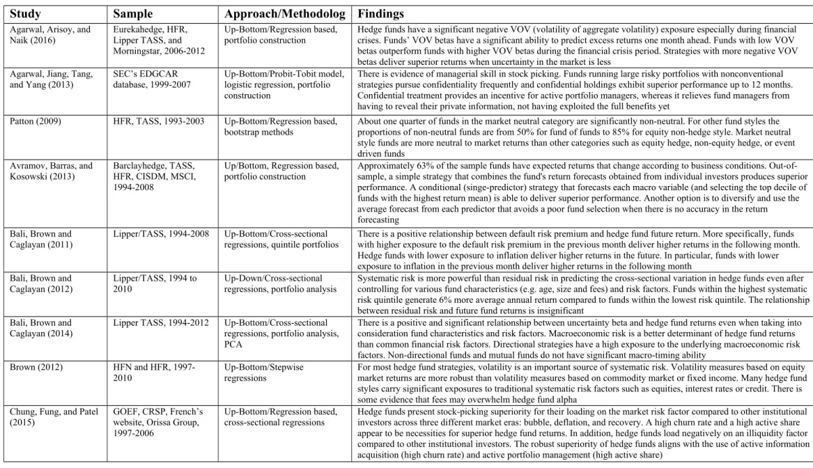
An in-depth study of the dependence between hedge fund returns and the S&P 500
index was carried out by Patton (2009) using the HFR and TASS databases from
1993 to 2003. He proposed five new neutrality concepts: mean neutrality, variance
neutrality tests showed that about one quarter of funds in the market neutral category
were significant non-neutral. For other fund styles the proportions of non-neutral
funds are from 50% for fund of funds to 85% for equity non-hedge. Market neutral
style funds were more neutral to market returns than other categories such as equity
hedge, non-equity hedge, or event driven funds. Overall, even for market neutral
funds there was significant and positive dependence between hedge fund returns and
market returns.
A closely related study with the above came from Bali, Brown, Caglayan (2012)
who examined how much the market risk, residual risk and tail risk justified the
cross-sectional dispersion in hedge fund returns, using the Lipper/TASS database
from 1994 to 2010. The authors separated the total risk into systematic and
fund-specific or residual risk components. Using cross-sectional regressions, univariate
and bivariate portfolio analysis they found that systematic risk was more powerful
than residual risk in predicting the cross-sectional variation in hedge funds, even
after taking into consideration various fund characteristics (e.g. fees, size and age).
Furthermore, funds within the highest systematic risk quintile generated on average
6% higher annual returns than funds within the lowest systematic risk quintile. These
results remained when using risk-adjusted returns as well. In addition the
relationship between residual risk and future fund returns was insignificant.
Dealing with Systematic Risk
As we mentioned, given that hedge fund strategies are not as neutral as they claim (at
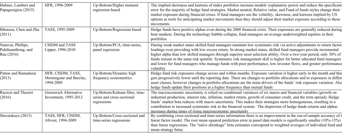
general macroeconomic environment that funds operate within. Ibbotson, Chen and
Zhu (2011) examined hedge funds’ alphas, betas and costs in a common framework.
They used the TASS database and the sampling period was from 1995 to 2009. Fees
were based on median fees - normally a 20 percent incentive fee and 1.5 percent
management fee. Using regressions with the S&P 500, U.S. intermediate-term
government bond returns and U.S Treasury bills, they broke down average hedge
funds annual returns of 11.3% into alpha (3.0%), beta (4.7%) and costs (fees,
3.43%). Their results showed that alphas were positive even during the financial
crisis in 2008. The only exception was in 1998. Their results showed that a typical
fund manager could add value in both bear and bull markets and their betas were in
general reduced during bear markets. For example, during the technology bubble
collapse fund managers underweighted equities in their portfolios.
A comparable study is from Bali, Brown and Caglayan (2011) who examined how
hedge funds’ exposures to various financial and macroeconomic factors could justify
the cross-sectional variations in hedge fund returns. They used the Lipper/TASS
database from 1994 to 2008. Their most important finding was that there is a positive
relation between hedge fund exposure to default risk premium and hedge fund future
returns. This could be interpreted as a meaning that risk premia on risky assets are
negatively correlated with present economic activity. For example, investors demand
higher expected returns in recessions and lower expected returns in booms when
holding risky assets. In a recession period, the default risk spread is high, so hedge
funds with higher exposure to the default premium are expected to give higher
returns. They also found that hedge funds with lower exposure to inflation derived
higher returns in the future. This has to do with uncertainty. As inflation rises, there
expect to observe a decline not only in hedge fund values but also in other financial
instruments. When inflation is stable and uncertainty is low then investors expect
those hedge funds and other financial instruments to have attractive returns. Overall,
non-directional strategies (such as Fixed Income Arbitrage and Convertible
Arbitrage) had lower variation and spreads in their exposures (beta factors) than
directional strategies (such as Global Macro and Emerging Markets).
Extending their 2011 work, Bali, Brown, and Caglayan (2014) proposed custom
measures of macroeconomic risk that could be regarded as measures of economic
activity, using the Lipper TASS database from 1994 to 2012. The macroeconomic
variables that the authors used were the default spread, term spread, short-term
interest rates changes, aggregate dividend yield, equity market index, inflation rate,
unemployment rate, and the growth rate of real gross domestic product per capital.
By using cross sectional regressions and portfolio analysis, they showed that
uncertainty betas can describe a significant proportion of cross section return
differences between hedge funds (two exceptions were unemployment and
short-term interest rate changes). More specifically, funds in the highest uncertainty index
beta quintile delivered 0.80% to 0.90% higher monthly returns and alphas compared
to funds in the lowest uncertainty index beta quintile. Moreover, the macroeconomic
risk was a more powerful determinant on hedge fund returns than other commonly
used financial risk factors (e.g. market returns, size, high minus low, momentum
etc.). In addition, through the use of principal component analysis, the authors
constructed an aggregate or broad index of macroeconomic risk whose first principal
component explained about 62% of the corresponding hedge fund return variance.
macroeconomic risk factors and non-directional strategies did not have significant
macro-timing ability.
Analogous to that study but emphasizing forecasting more was the study by
Avramov, Barras, and Kosowski (2013). They developed a unified methodological
framework to asses both in-sample and out-of-sample hedge fund returns
predictability based on macroeconomic variables, using the Barclayhedge, TASS,
HFR, CISDM, and MSCI databases from 1994 to 2008. Beginning from in-sample
analysis, approximately 63% of the sample funds had expected returns that changed
according to business conditions. They used five macro variables (default spread,
dividend yield, VIX index, net aggregate flows in the hedge fund industry) and
found that returns predictability was widespread across different hedge fund
strategies, consistent with economic intuition. A conditional (singe-predictor)
strategy that forecast each macro variable (and selecting the top decile of funds with
the highest return mean) was able to deliver superior performance. By diversifying
across forecasts, the combination strategy is more sufficient when return forecasts
are not sufficiently accurate, thus avoiding a poor fund selection.
Racicot and Theoret (2016), using strategy indices from the Greenwich Alternative
Investment database from 1995 to 2012, examined the behaviour of the
cross-sectional dispersions of hedge funds’ returns, market betas and alphas during times
of macroeconomic uncertainty. In their model they used the three Fama and French
(1993) factors and the Fung and Hsieh (1997, 2001, 2004) lookback factors.
Macroeconomic uncertainty was modelled using the conditional variances of six
macro and financial variables (growth on industrial production, interest rate,
Kalman filter technique they found that hedge fund market beta reduces with macro
uncertainty. This makes their strategies more homogeneous, resulting in a
contribution to the increased systematic risk of the financial system. The dispersion
of hedge funds returns and alphas increases during times of rising macroeconomic
uncertainty.
Relevant to the above study is the study of Namvar, Phillips, Pukthuanthong, and
Rau (2016) who used the CISDM and TASS Lipper databases from 1996 to 2010.
Using Fung and Hsieh’s (2004) factors in their model with PCA, time series and
panel regressions, they examined the prevalence and the determinants of the
systematic risk management (SRM) skill of fund managers and its effect on funds’
performance over time. They used the spread between the AA and BB corporate
bond index yields to define the strong, medium and weak market states. They found
that during weak market states, skilled fund managers maintain low systematic risk
via active adjustments to return factor loadings, even though that provides low
excess return. In strong market states, skilled fund managers provide higher alpha
than low skill managers through their superior asset selection ability. More
experienced or more educated fund managers present higher SRM skill. Moreover,
SRM is lower for managers who manage funds with distress indicators (e.g. low
investor flows or poor performance).
Higher Moment Risk and Refined Factors
In this sub-section we present some studies that try to explain hedge fund
databases, from 2006 to 2012, investigated whether uncertainty about volatility of
the market portfolio could explain the performance of hedge funds, both in the
cross-section and over time. They measured uncertainty about volatility of the market
portfolio with the volatility of the aggregate volatility (VOV) of equity market
returns. They constructed an investable version of this measure by calculating
monthly returns on lookback straddles on the VIX index. They found that there was
negative relationship between VOV exposures and hedge fund risk adjusted returns;
however, this was not homogenous across all hedge fund strategies. They also found
that the VOX negative exposure was a significant determinant of hedge funds returns
at the general index level, at different strategy levels, and at the individual level as
well. Strategies with less negative VOV betas outperformed strategies with more
negative VOV betas during banking crisis period. Conversely, strategies with more
negative VOV betas delivered superior returns when the uncertainty in the market
was less. Also funds’ VOV betas had a significant ability to predict excess returns
one month ahead.
Related to the above study was that from Hubner, Lambert and Papageorgiou (2015),
who modelled hedge fund returns on a conditional asset pricing model using the
information content of market skewness and kurtosis. They used the HFR database
from 1996 to 2009. They described the dynamics of the equity hedge, event-driven,
relative value, and fund of funds styles and in their model considered the location,
trading and the higher-moment factors. Within this framework they investigated the
effect of the implied moments retrieved from the US equity markets and more
specifically from the option-implied higher moments. The implied skewness and
kurtosis of index portfolios increased the model’s explanatory power and reduced the
Fund of Funds change their market exposure during financial crises. The authors
recognized that an extension of their framework to other market types and locations
would provide extra explanatory power to their model.
There are studies that use high frequency econometrics or refined statistical methods
to choose the appropriate factors. For instance, Patton and Ramadorai (2013)
proposed a new performance evaluation method that was based on Ferson and
Schadt’s (1996) model (a customized conditional model for mutual funds
incorporating lagged information variables). That model was able to capture
higher-frequency variations in hedge funds’ exposures. They used the HFR, CISDM, TASS,
Morningstar and Barclays databases and the sample period was from 1994 to 2009.
In their factor model that included a simulation process, they used daily hedge fund
(index) returns in relation to monthly hedge fund (individual) returns. They observed
similar parameter estimates across the two sampling frequencies. Furthermore, hedge
funds exposures varied across and within months. Moreover, they discovered
patterns where the exposure variation was higher early in the month (immediately
after the reporting date) and then got progressively lower until the reporting date. In
addition, they found changes in portfolio allocations (weights) (that ultimately led to
exposure changing) rather than changes in exposures to different asset classes and
also a tendency to cut positions in response to significant market events (such as
sharp changes in market returns or volatility). The authors’ results showed that hedge
funds, contrary to mutual funds, responded very quickly, were very flexible and
adapted to any market triggers.
1997 to 2010. In order to better estimate hedge funds fees, betas and alphas he
suggested a framework that monthly returns be drawn from the following influences:
fees (management and incentive fees) and four simple systematic risk factors. Those
were volatility, leverage and two other more traditional factors such as equities,
credit, interest rates, or commodities. For most fund strategies, volatility is the most
important source of systematic risk. Brown applied stepwise regressions to various
style or aggregate indices because of the need to customize performance benchmarks
to different styles. He found that many hedge fund styles carried significant
exposures to traditional systematic risk factors such as equities, interest rates or
credit. Due to the fact that incentive fees are computed on total returns, there is a
potential that abnormal returns attributed to those systematic exposures may
overwhelm hedge fund alpha. Thus, fund managers may get paid for simple passive
market exposures. Those problems of charging incentive fees on simple market
exposures extend to most hedge fund styles and therefore constitute a barrier to their
efficient usage.
Lastly, Slavutskaya (2013) improved the out-of-sample accuracy of linear factor
models by combining cross-sectional and time-series information (panel data
methods) for groups of hedge funds with similar investment strategies. She used the
TASS, HFR, CISDM, and Alvest databases from 1994-2009. She suggested that
current factor models are over-parameterized which results in unstable estimates.
The “shrinkage” estimate, which is the trade-off between the individual estimates
and the common mean estimate (the average risk exposure of a particular hedge fund
style) provided a more accurate estimate. More specifically, she found that the root
mean squared monthly error in panel data models was 10-15% smaller than in linear
the use of cross-sectional beta estimates assumed that all funds had the same risk
exposures for a given time.
Holdings/SEC filings
A study that focused on the funds’ security holdings and stock-picking was that of
Chung, Fung, and Patel (2015). They examined whether hedge funds deliver
consistent superior performance by focusing long-equity holdings. They used four
databases: GOEF, CRSP, data from French’s website, and that of Orissa Group from
1997 to 2006. By focusing on the characteristics of returns associated with
long-equity picks of hedge funds and other institutional investors, they showed that hedge
funds presented stock-picking superiority on their loading on the market risk factor
compared to other institutional investors across three different market eras: bubble,
deflation, and recovery. Moreover, high information acquisition (high churn rate)
and active portfolio management (high active share) appeared to be necessities for
the superior returns of hedge funds relative to other institutional investors.
Related to the above study is the paper by Agarwal, Jiang, Tang and Yang (2013)
who examined the “confidential holdings” from hedge funds which are amendments
to Form 13F (SEC’s requirement of quarterly holdings report for funds with over
$100 million in qualifying assets), using the SEC’s EDGAR database (1999-2007).
The authors incorporated and compared confidential holdings’ performance to
original holdings’ performance of fund managers’ portfolios providing a clear
picture of the stock-picking ability of hedge funds. They showed that confidential
benefits of their investments. Funds managing large risky portfolios with
nonconventional strategies (e.g. higher idiosyncratic risk) pursue confidentiality
frequently and confidential holdings exhibit superior performance from 2 to 12
months. Although the conventional 13F databases which ignore confidential
holdings may be biased, this bias is small when considering aggregate institutional
holdings in public companies. However this is a significant omission when analyzing
position changes of individual institutions or in response to certain events.
The above studies using additional factors and statistical techniques examined in
detail systematic risk and performance, and the way they change according to
financial conditions or holdings. However, more work is needed look at the time
variation of hedge fund performance attribution. This is an issue that can better be
captured with the identification of the structural breaks within the underlying
models, as presented in section 5.3.
5.3 Alternative Approach
In this section we present studies that have addressed different methodological issues
and tried to identify structural breaks in hedge fund returns. These studies focus on
the model uncertainty and its different behaviour when describing hedge fund
returns. As with the up-bottom approach, these studies also tend to use more
advanced econometric techniques.
We begin with Bollen and Whaley (2009) who used the CISDM database from 1994
to 2005. They ran an optimal change-point regression model that allowed risk
exposures to switch (although they implemented it using just one
exposures. In order to select the most appropriate subset of available factors they
first selected a subset of factors that maximized the explanatory power of a constant
parametric regression by using the Bayesian Information Criterion. The change-point
regression model performed better overall compared to the stochastic beta model,
showing that approximately 40% of the hedge funds in their sample presented a
significant shift in risk exposures. Moreover, for live funds, switches tend to take
place early in the fund’s life, whereas switcher funds tend to outperform
non-switchers funds. Overall, time-varying risk exposures presented better estimates of
funds’ alphas and could make better hedge fund returns predictions.
Giannikis and Vrontos (2011) used the HFR database from 1990 to 2009 to examine
the non-linear risk exposures of hedge funds to various risk factors. Their analysis
revealed that different strategies exhibited non-linear relationships to different risk
factors and that a threshold regression model incorporating a Bayesian approach
improved the ability to appraise hedge fund performance. They used the Bayesian
approach to identify the relevant risk factors (instead of stepwise regression or
performing other statistical criteria) and at the same time detect possible thresholds
in the model. The Bayesian methodology solved two problems of the regression
models: first, the uncertainty of the set of the risk factors and, second, the number
and the values of the appropriate thresholds. This was a probabilistic approach
incorporating prior information – inferences appropriate to the underlying datasets.
Finally, different hedge fund strategies presented different timing abilities.
One more recent innovative study was from Jawadi and Khanniche (2012). They
in a non-linear framework, and more specifically the smooth transition regression
method. They found that the dynamics of hedge funds returns realized significant
asymmetry and non-linearity in relation to the market return, showing that they
changed and differed asymmetrically with respect to different financial conditions.
Furthermore, hedge funds exposures varied over time depending on the strategy and
regime. They advocated the superiority of non-linear models to capture the evolution
of hedge funds exposures, especially during periods of financial crisis.
In the same year, Billio, Getmansky and Pelizzon (2012) examined hedge funds
exposures using regime-switching beta models on data from the Credit
Suisse/Tremont database from 1994-2009 (hedge fund indices). They noticed that
hedge funds had non-linear exposures not only to the equity market risk factor, but
also to the liquidity risk factor, volatility, credit, term spreads and commodities.
Also, hedge funds changed their exposures when dealing with up, down, or tranquil
regimes. Furthermore, they found that the S&P 500, Credit Spread, Small-Large and
VIX (measure of volatility in S&P 500 index options – Chicago Board Options
Exchange) were common hedge fund factors, especially in a falling market. The
estimated exposures were unaffected even when authors de-smoothed the returns.
A related to the above study was from Akay, Senyuz and Yoldas (2013) who
examined hedge fund industry contagion and time variation in risk adjusted return
(alpha), using the Dow Jones Credit Suisse Hedge Fund Indices database from 1994
to 2010. They used a Markov regime switching model and found three regimes that
could capture hedge fund returns dynamics: the first was the crash state with large
negative mean and extreme volatility, the second regime was a low mean and high
They also found evidence for a decline in risk adjusted returns for most investment
strategies especially after the stock market crash in 2000. Moreover, they found that
co-movement in hedge funds returns, after counting for common risk factors, was
not only restricted to times of extreme financial turbulence. Last but not least, they
linked the probability of observing the crash state to liquidity proxies and panic,
measured by the VIX index and found that both played a significant role in leading
to contagion.
A final study is from O’Doherty, Savin, and Tiwari (2015), using the Lipper TASS
database from 1994 to 2011, implementing a pooled benchmark model by combining
(with different weights) five linear models: five equity factors, three fixed income
and commodity factors, three global factors, the five Fung and Hsieh (2001) trend
following factors, and the four Agarwal and Naik (2004) option-based factors. Their
optimal pool was based on the score log which was a measure of the conditional
performance of a factor model, regarding its ability to track the monthly return for a
given hedge fund. The authors verified that the above factors of the models capture
hedge funds’ exposures; in addition, their optimal pooled benchmark mitigated the
(benchmark) error of these factor-based attribution models. Also the model pooling
approach had more predictive power for failures among the funds in their sample
than other performance attribution models.
To sum up, several studies that follow the bottom-up approach have examined hedge
fund performance as a non-linear payoff of hedge fund returns in relation to market
returns. However this method is not easily understood or implemented by investors.