Transmission matrices and lumped parameter models for continuous systems

Thesis by

Richard Dale Rocke

In Partial Fulf:lllinent of the Requirements for the Degree of

Doctor of Philosophy

California Institute of Technology Pasadena, California

1966

ACKNOWLEDGMENTS

The author desires to gratefully acknowledge the guidance and encouragement given by his former advisor, the late Professor

C. E. Crede, during the early phases of graduate work.

The many ideas and suggestions provided by Dr. Sheldon Rubin during the entire course of this investigation have been sincerely

appreciated.

The author is especially grateful to Professor D. E. Hudson, his present advisor, for the guidance, encouragement, and valuable suggestions provided during the course of this work and the prepara-tion of this manuscript.

The author is. further indebted to the Hughes Aircraft Company for the Doctoral Fellowship and other generous financial aids provided, to the California Institute of Technology, and to the National Aero-riautics and Space Administration for partial support of this wor~ under

Contract No. NAS 8-2451.

ABSTRACT

The use of transmission matrices and lumped parameter model's for describing continuous systems is the subject of this study. Non-uniform continuous systems which play important roles in practical vibration problems, e.g., torsional osdllations in bars, transverse bending vibrations of beams, etc., are of primary importance.

A new approach for deriving closed form transmission matrices is applied to several classes of non-uniform continuous segments of one dimensional and beam systems. A_ power series expansion method is presented for determining approximate transmission matrices of any order for segments of non-uniform systems whose solutions can not be found in closed form. This direct series method is shown to give results comparable to those of the improved lumped parameter models for one dimensional systems.

Four types of lumped parameter models are evaluated on the basis of the uniform continuous one dimensional system by comparing the behavior of the frequency root errors. The lumped parameter models which are based upon a close fit to the low frequency approxima-tion of the exact transmission matrix, at the segment level, are showi:.i· to be superior. On this basis an improved lumped parameter model is

recommended for approximating non-uniform· segments. This new . model is compared to a uniform segment approximation and error

CHAPTER

I

II

III

IV

TABLE OF CONTENTS

TITLE NOMENCLATURE

. INTRODUCTION

1. 1 Contents of Thesis TRANSMISSION MA TRICES

2. 1 Description

PAGE

1 2 4 4 2, 2 Direct Derivation of Transmission 9

Matrices

SYSTEMS GOVERNED BY THE ONE DIMENSIONAL WAVE EQUATION

3. 1 Comparison of Different Physical . Systems

3. 2 Transmission Matrices for Continuous Systems

12

12-15

3. 3 Investigation of Lumped Parameter 19 Models

3. 4 Linear Taper Model 42

3. 5 Optimum Segmenting with the 69 Linear Taper Model

BEAM ELEMENTS

4. 1 Lumped Parameter Models for Uniform Continuous Beams 4. 2 Transmission Matrices for

Non-Uniform Continuous Beams

82 82

CHAPTER

v

.

VI

TITLE.

POWER SERIES EXPANSION OF TRANSMISSION MA TRICES

5.1 Method Description 5. 2 Illustration

SUMMARY AND CONCLUSION APPENDIX A

APPENDIX B APPENDIX C APPENDIX D REFERENCES

PAGE

99

99

102 109 114

119

[A]

A(x}

. A 0

B

b

c

c

D.(x} 1

[E)

E

NOMENCLATURE

=

matrix (n X n) which characterizes a system

= cross sectional area expressed as a function of x

=

cross sectional area at the input end of a segment

= cross sectional area at the output end of a segment

=

Nf3

= width of a rectangular cross section

= variable used to .control segment lengths

= constants in the transmission matrix for a beam i, k=l,2,3,4

= velocity of sound

=

ith differential operator with the independent variable x

= transmission matrix (n X n} for a uniform continuous system

=

Young's modulus

EI(x) - beam bending stiffness expressed as a .function of x

EI = beam bending stiffness at the input end of a segment 0

= non-dimensional frequency root error for the vth mode with N· segments

F = force

f = 1

;g

g 1

+

f

G

=

shearing modulus

h = height of a rectangular cross section

I ±n J ±n K ±n k. 1

[ L]

L

[M]

M N n p r r

[ T]

u v y :1:n·

Y(x)

O!

f) l

E

E ••

lJ

= modified Bessel function of the first kind, of order n

= Bessel function of the first kind, or order n

= modified Bessel function of the second kind, of order n

.th . '

= i spring constant

= transmission matrix (n X n) for lumped parameter models

=length of an element composed of N segments

= length of one segment (or increment)

= transmission matrix (n X n) derived by power series expan-sion method

= point mass (except where noted in Appendix D)

= number of segments

= constant for controlling cross sectional variation of beams

= constant for controlling cross sectional area variation

= radius of circular cross sections

= radius of gyration

= transmission matrix (n X n) for non-uniform continuous systems

= rectilinear displacement

= rectilinear velocity

= Bessel functions of the second kind, of order n

= admittance type element in the [A ] . matrix expressed as function of x

= ff)

= w

J

p/E

= matrix norm

i) = subdividing parameter for lumped parameter models ~ = slope parameter

p = mass density

<J' = stress {force/area)

1

µ

=

2

If

J!fl

[~~:]

4

.v =mode number

l\J

-

state vector {column vector)

A general theory for vibration problems involving continuous systems has existed for many years. However, the number of

prob-lems which are exactly solvable analytically is very small, e.g.,

uniform and some simple non-uniform systems. Therefore, other techniques, which give approximate solutions to continuous systems, have been extensively investigated. These methods provide solutions to many practical vibration problems which do not fit into the category of being exactly solvable.

One method, which has been especially emphasized since the

advent of large computers, is the lumped parameter approximation

whereby the continuum is replaced by a finite N degree ·Of freedom system composed of lumped elements, i.e., massless springs, point masses, etc. This technique was first applied by Lagrange [ 1

J

and

Rayleigh[ Z] in studying the vibrating string. Duncan[ 3

J,

using a lumped parameter model attributed to Lagrange, was one of the first

to study the behavior of errors resulting from lumped parameter

ap-proximations .. Livesley[ 4

J,

Gladwell[ 5

J,

and others[b,?,B]have evaluated lumped parameter approximations of uniform continuous beams using many different models.

Transmission matrices, which have been applied to mecha ni-cal vibration problems only in recent ye·ars, provide another approach

for describing continuous systems in either an exact or approximate

description of four terminal electrical networks in which case the method is commonly designated "four pole parametersn. Molloy[ 9 ] was one of the first to systematically apply four pole parameters to acoustical, mechanical, and electromechanical vibration problems. Pestel and Leckie[ lO] have catalogued transmission matrices for uniform elastomechanical elements up to twelfth ord.er. R bu in . [ 11] has extended the application of transmission matrices through a

completely general treatment.

1. 1 Contents of Thesis

The objective of the present study is to investigate more thoroughly several aspects of the application of lumped parameter and transmission matrix approaches to vibration problems, in par-ticular, those problems which involve non-uniform continuous systems.

In Chapter II transmission matrices and their derivation are briefly discussed.

fhghts [ l Z]. Models based on the one dimensional wave equation

similar to those to be treated in Chapter III were used to describe

structural components and fluid lines in the analysis of this missile

vibration problem.·

Chapter III also contains a presentation of transmission

matrices for three classes of non-uniform continuous cross sections

and the transmission matrix technique is used to evaluate the error

behavior of four types of lumped parameter models used to

approxi-mate the uniform continuous system. A new lumped parameter model

is proposed for non-uniform systems and for one particular case,

the linear taper model, the lumped parameters are defined. In

addi-tion, the effect of varying segment lengths is ptudied.

Chapter IV includes a surnmary of various lumped parameter

models which have been used to approximate uniform beams.

Trans-mission matrices for three groups of non-uniform continuous beams

are derived.

A power series expansion method for obtaining transmission

matrices which are low frequency approximations for non-uniform

continuous syst.ems of any order is presented in Chapter V.

Finally a summary of the work presented herein, and

2. 1 Description

CHAPTER II

TRANSMISSION MA TRICES

The transmission matrix describes the manner in which

sinusoidal forces and motions are transmitted through a linear elastic

· element during steady state conditions. All consideration .of the

dif-ferential equations describing the element is contained within the

derivation of the 'transmission matrix and the approach is equally

applicable to lumped parameter or continuous systems.

A general transmission element is shown in Fig. 2. 1. 1. The

state vector. denoted by l);' is a column vector consisting of forces

and velocities or displacements. The transmission matrix relates

the state vector at the input to that at the output of the element. The

form of the transmission matrix which will be used herein is:

{1.j;

}input - [ T] {l.j; }output (2.1.1)

where [ T

J

is commc:mly designated the "forward transmission ·

matrix". The sign convention to be used, see arrows in Fig. 2. 1. 1,

has positive directions for forces applied

EY

the output the same as

those for forces applied to the input.

·When a line of elements or segments are in an end-to-end or

chain like arrangement,· which is the situation for which this approach

is best suited, the transmission matrices for the individual segment

r-z

lJJ ti;:' ..:! lJJ ....J

tJ

_lJJ

r-

I

2

0

::>

I

(/)

a...

r-(/)

::>

I

~

0

(/) ~

I

z

~

<C

"-v--'

~

a::

i-<( LL

0

.

z

(\J

Q

0

·

·-

-

_{I- LI..}

<{

r-z

w

(/)

w

a::

i

-l\

a..

{l\J } = [ T ]

{~ }

1 1 z

{l\J

}=

(T ]

{l\J}

z z . 3

and for the total chain of segments:

.

{l\J }

= [ T ] [ T ] . . . • . . [TN ]{lj!N}

1 1 z -1 (2.1.2)

This simple result is obtained because the state vector at the input of any given segment is equal to the state vector deliyered by the output of the preceding segment. This result will be used in the following chapters to obtain the overall transmission matrix for a system com-posed of N segments.

Another way to write the state vector and transmission matrix is in partitioned forrr;i. where the state vector becomes:

(2. 1. 3)

and the transmission matrix is:

A1B [T]=

---i---[

. I ]

. C: D

For one dimensional systems, e.g. , the longitudinally vibrating rod,

F is the force, V is the velocity, and the submatrices in

p p

Eq. ( 2. 1. 4) reduce to scalar quantities. For the simple transverse

bending beam, ,however, the transmission matrix is fourth-order,

shear force

bending moment

rectilinear velocity

rotational velocity

and the submatrices in Eq. ( 2. 1. 4} are 2 X 2 matrices. Pestel and

Leckie[ lQ] have catalogued transmission matrices for various

uni-form elastomechanical elements which have transmission matrices

up to twelfth-order (12 X 12}.

The elements of the transmission matrix are not independent

and as a consequence of reciprocity it has been shown [ 11] that the

square submatrices of Eq. (2. 1. 4} must satisfy:

(2. 1. 5)

.where:

I

[I]

=the identity matrix, and

[A]T =the matrix transpose of [A]

Equation (2. 1. 5) provides an excellent means of checking the validity

of derivations of transmission matrices.

lumped parameter models in Chapter III, are important character-istics of unda_mped linear elastic systems which can be obtained

through the use of transmission matrices. The transmission matrix, by definition, is independent of boundary conditions and is a function of frequency, w. Upon substituting the appropriate boundary con-ditions for a system into the input and output state vectors of Eq. (2. 1. 1), a frequency determinant can be obtained. A simply sup;.. ported beam, for example, with the boundary conditions included in the state vectors is described by:

which gives:

v.

1

0 0

.

</>. 1

=

T ..

lJ

.

O'=VT +c/>T

O Zl 0 M

.

O=VT +c/>T

. 0 31 0 34

v

0

(2. 1. 6)

(2. 1. 7)

For a nontrivial solution of Eqs. (2. 1. 6} and (2. 1. 7} the determinant of the T.. coefficients must be zero, that is,

lJ

T

T

Zl M

=

0

T

T

31 34

which define the natural frequencies. To obtain normal mode fre-quencies of one dimensional _systems which are described by second-order {2 X 2) transmission matrices the above process reduces to finding zeros of single T.. elements, e.g., the natural frequencies

iJ

of a free-free rod are given by the zeros of the T

lZ term.

Having determined the naturci..l frequencies, the corresponding normal mode shapes can also be obtained. This is accomplished. by relating the nonzero components of the input state vector to one reference component. Then the state vectors are determined at other points through the system, in terms of the one reference com-ponent, by applying the. transmission matrix which relates the input to the point in question. The determination of normal mode frequen-cies and mode shapes in this manner has been demonstrated by Molloy[ 9 ], Pestel and Leckie [ 1 OJ, Rubin [ l 3.], and others in tp.eir application of transmission ·matrices to mechanical vibration prob-lems.

2. 2 Direct Derivation of Transmission Matrices

Methods used in finding transmission matrices, in the past, have. v·aried according to the preferences of the users. These meth-ods have proven satisfactory for simple lumped parameter or lower-order uniform continuous systems, but become cumbersome when used for non-uniform and higher-order systems because. of the

. d 1 b . . 1 t' R 1 h R b' ( l 4

J

require a ge raic manipu a ions. ecerit y, owever, u in

algebra and results directly in differential equations for the elements

of the transmission matrix. This approach will be summarized in this section and· its application demonstrated in Appendices A, B,

and D.

'

.

.

[10]

In general, the state vector is usually known · to satisfy

a differential equation of the _form:

~

{tJ;(:x;)}=

[A(x)]{ljJ(x)} (2. 2.1)

The [A(x)

J

matrix is entirely determined by the differential

equa-tions which govern a· dx increment of the system (see Appendix A or D). By definition of the forward transmission matrix:

{ljJ(O)} = [T(x)J {ljJ(x)} (2. 2. 2)

Differentiating Eq. (2. 2. 2) _with respect to x gives:

I I

0 = [ T (x)] {ljJ(x)} + [ T(x) ]{ljJ(x)} . (2. 2. 3)

I

However, {ljJ(x)} can be replaced using Eq. (2. 2.1); hence, reduc-ing Eq. ( 2. 2. 3). to:

I

0

=

[T (x)]{ljJ(x)}+ [T(x)][A(x)]{ljJ(x)}

which upon elimination of {ljJ(x)} gives:

~

[T(x)]

=

-[T(x).][A(x)] (2. 2. 4)

becomes:

(T(O)] =I the -identity matrix. (2.2.5)

Substituting this result into Eq. (2. 2. 4) gives:

I

(T (O)]

=

-(A(O)] (2. 2. 6)

Differentiating Eq. (2. 2. 4) with respect to x and using Eqs. (2. 2. 5)

It

and (2. 2. 6) results in [ T (0)]. This process can be continued to

obtain as many initial conditions as required to evaluate constants

which arise in solving Eq. ( 2. 2. 4); hence, the formulation of the

CHAPTER III

SYSTEMS GOVERNED BY THE ONE DIMENSIONAL WAVE EQUATION

3. 1 Comparison of the Different Physical Systems

The one-dimensional wave equation mathematically describes a group of uniform continuous systems. The following three vi

bra-tion problems have this identical mathematical formulation with

suitable interpretation of properties. 1. longitudinal vibration of rods,·

2. torsional vibration of bars, and

3. acoustical vibrations in tubes.

·Another system belonging to this category is the electrical transmission line, which has been treated rather extensively by Pipes . [15,16,17]. . . The transmission line will not be specifically in

-eluded herein, but some of the resulting transmission matrices and

lumped parameter models could be directly applied to this problem. When considering the cross sectional properties of the above ·

systems to be non-uniformly distributed, the governing differential

equations in each case are all similar; and each system under

steady-state sinusodial conditions is described by a similar second-order ( 2 X 2) transmission matrix of the following form.

\l [

ljJ

=

T 11 T lZ ] { } ljJ

input T 21 T 22 output

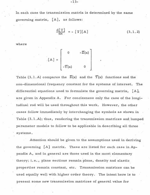
In each case the transmission matrix is determined by the same

governing matrix, [A], as follows:

where

d[T]

~

.

[A]

=

= -

[T][A]

0 -Z(x)

-Y(x) 0

( 3. 1. 2)

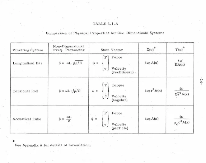
Table (3. 1. A) compares the Z{x) and the Y (x) functions and the

non-dimensional frequency constant for the systems of interest. ·The differential equations used to formulate the governing matrix, [A],

are given in Appendix A. For conciseness only the case of the

longi-tudinal rod will be used throughout this work. However, the other cases follow immediately by interchanging the symbols as shown in Table (3. 1. A); thus, rendering the transmission matrices and_ lumped parameter models to follow to be applicable in describing all three

systems.

Attention should be given to the assumptions used in deriving

the governing [A] matri~. These are listed for each case in

Ap-pendix A, and in general are those used in the most. elementary

theoxy; i.e., plane sections remain plane, density and elastic

properties remain constant,, etc. Transmission matrices can be used equally well with higher order theory. The intent here is to

Comparison of Physical Properties for One Dimensional Systems

Vibrating System

Longitudinal Bar

Torsional Rod

Acoustical Tube

....

...

Non-Dimensional Freq. Pa:i;ameter

f3

= wL

JPfE

f3

= wL Jp/G

f3

= wL

c

See Appendix A for details of formulation.

State Vector

ljJ

=

{Fv} Force

Velocity (rectilinear)

-ljJ

=

Torque

Velocity (angular)

ljJ = {vF} Force

Velocity

(particle)

...

Z(x) ...

iwp A(x)

iwpr2 A(x)

iwp A(x)

....

Y(x).,.

iw EA(x)

iw

Gr

2 _A(x)

iw

...

describing non-uniform systems and in particular to use them to

improve lumped parameter modeling of continuous systems. These

principles can be sufficiently demonstrated using the elementary theory.

3. 2 Transmission Matrices for Continuous Systems

The parameter des cri birig the spatial dependence in the

governing matrix, [A

J,

is the area, A(x). To obtain a transmis

-sion matrix useful for describing many non-uniform systems requires

selection of a general function to represent the variable area. This

function must be general to represent many useful cases but of a

form which will lead to closed form solutions. One such function is:

z

-1

A(x) =A

0 (l+ax) p (3.2.1)

where

a = some suitable constant and

p = an integer or non-integer.

Another useful function for exponentially tapered sections is:

where

z (x/x ) A(x) =A e 0

0

x = some suitable constant. 0

(3. 2. 2)

Equation (3. 2. 1) with a convenient coordinate transformation

leads to differential equations for the transmission matrix elements·

d2 T.. dT ..

x2 lJ + ax ~d 1 · + bx2 T .. = 0

dxz . x lJ

It is well known that this equation with variable coefficients has

solu-tions in terms of Bessel funcsolu-tions. The exponential t_aper leads to

second-order differential equations with constant coefficients of the form:

d2T.. dT ..

-1

""'J

+

a --.-:.Ld 1

+

b T. . = 0

dxz x . lJ

which can be easily solved.

Using the two area functions given in Eq. (3. 2. 1) and (3. 2. 2) and following the basic approach outlined in Section 2. 2, general

transmission matrices can be derived· for a broad group of non-uniform continuous elements. The derivation of the general matrix

elements for three specific cases (p = an integer, p

I

an integer, and the exponential taper) is given .in Appendix B. The resulting

trans-mission matrices for these three cases are given below:

Case I A(x) =A (l+ax{ p-l p = 0 or an integer 0

l -p

T (£) =( fg}

.!._

{Y · (fj3)J (gl3)-J (fj3)Y (gl3)}

11

x

-p i -p -p l -p

T (1)

12 . l {Y (fj3)J (gf3)-J (fj3)Y (gf3)}

X P P P P .

T (l) = -

~rA

f.

E]

(fg). 1-p

.!._

{Y (fj3)J (gj3)-J. (f(3)Y (g.f3)}

21 I-'

·

x

p-1 p-1 p-1 p-1

0 ' I

p .

T (£) =(;}

.!._

{Y . (ff3)J (gj3)-J .(fj3)Y (gf3)}

~

I-=>

0...

...

:::>

0

,--A-. LL >

'-v-1

-

~

-

<(

..

Ll.J

..

Q,,

<l.

o

I-:::>

a..

z

,--A-. LL > '-w-J ' ) (

_J

r-z

w

~

w

....J

LLJ

(.)

-...

(/)

<( --:

....J

C\J

w

r0

(..9

~

u..

X

=

2/ ir£f3 independent of 11_{p" in this case.}

Case II A(x) -- A (l+ax)zp-l -1- 0 · t

0 p T or an in eger

1-p

T (1) = (gf)

l_

{Jp(ff3)J (gj3)+J (£f3)J (gf3)}

11

x

i-p -p p-1

T (J..) =

.1..[E~o]

(Kf)P

..!_

{J (ff3)J (gf3)-J (£f3)J (gf3)}

lZ lW Jt.. X p . -p . -p p

T (.e)

z l

~

[AoJ..E

l

(.&)

l -p Xl {J (£f3)J (gf3)-J J . (gf3)}

tJ

J

1 l ""'P . p-1 p-1 l -p

T (£) = (Kf )P

l_

{j

(£ f3)J (g f3) +J (£ f3)J {g

13)}

.

zz

x

i -p p p-1 -p

2

X = ir£f3 sin (pir)

In Cases I and II the following definitions are appropriate (see Fig.

3. 2.1):

s

= a slope parameter =

A

=

area at the input end of the element 0

A .R.

=

area at the output end of the element

£

=

l/s

a

=

s/J..

g

=

£

+

1 and f3

=

w1

J;/E'

For systems with circular cross sections:

S·

= ( r n - r ) / r

Jt.. 0 0 where r

0 and r 1 are the radii. at the input and output ends,

Case III

T

11

(£)

T

12. {l)

T

2.1

(£)

T (£) zz

where

= e

z (x/x )

0

A(x) =A e 0

-i. Ix

( co s( 'Y .£ )

+

I 0

'YX

0

sin( 'Yi.).

£/x

(A

0E) (

~~

)

sin(~

1

)

0

e

=

lW

-.R./x

13z

0(

e i

-

-

_{iw pA}

0'Y

i.

/x

= e 0 ( cos('Y.R.)

..: l/x

z

0

) sin('Yi.)

- - 1- sin("Yi.))

-'YXO

and the other terms are identical to those used in Cases II and III.

This element exhibits a cut-off frequency,

13z

=

1

/x z.

l 0 When

{3:

<

l /x~, oscillations do not occur in the element; and when

13:

>

l /x

0 2

, mechanical oscillations do exist. Thus, this element be-hci.ves as a high pass rµechanical filter.

3. 3 Investigation of Lumped Parameter Models

The determination of eigenvalues and eigenfunctions for co

n:-tinuous systems is generally_ a difficult problem. The approach of

using transmission matrices to piecewise describe a continuous system has been previously discussed in Section 2. 1, and a general

-

0

-.Q

--

c

-

·

CJ)

....J

w

0

0

systems has been given in Section 3. 2. Another more commonly used

approach· is to replace the continuum by a discrete N degree of

free-dom system composed of lumped parameters. It has been shown [ 2]

that the behavior of the discrete N degree system approaches that of

the continuous system in the limit as N - oo , and it is on this basis

that this method is justified. However, the degree to which the finite

system approximates the· continuous is often uncertain even though this

technique is widely used. The main goal in this and the following

. .

sections is to formulate some generalizations as to which lumped

parameter models should be used, how they should be employed, and

what accuracies can be expected upon using the models.

Three models that have been used previously are given in

Fig. (3. 3.1). In the first model, which was first used by Rayieigh[2

J,

the total mass. of each of the N increments into which the rod has

been segmented is further divided into two equal masses concentrated

at each end of a spring which represents the stiffness of the increment.

The second model, which has been attributed in the literature [ 18] to

Lagrange, has been investigated to some extent by Duncan [ 3] and is

some times referred to as Duncan's model. This model has the mass

of the increment concentrated at the center and equal springs on each

side. The third model, which is used to a large e::l<i;ent in practice, has

the mass concentrated at one end of a spring.

To critically examine the usefulness of these models requires

a mathematical approach. which allows the formulation of the problem

-22-system representation as a function of the number of increments. A

method commonly used by some is the finite difference approach. The

approach used herein is that of .the transmission matrix, which was

chosen for the following reasons:

1. This method allows complete freedom to choose

incremental models in any form.

2. This metho.d provides a means of determining how well the models represent the continuum at

the incremental level. Also, the accuracy of

representing a total element by N increments

of a given model can be evaluated.

3. The method allows for an analytic treatment of

uniform systems and is easily extended to include

non-uniform systems.

3. 3. 1 Model Comparison on the Incremental Level

The first comparison for the models shown in Fig, (3. 3. 1) is

to determine how well the tran.smis sion matrix for each agrees with that of the contimious uniform system for one increment of length .R..

This should give some insight into what model will best describe an

overall continuous uniform element 'composed of N increments.

Using the state vector form involving force and displacement, the

transmission matrix for the continuous uniform rod is (see

cos (13)

(E]

=

fl.

A--:E

0

sin(f3) 13

A E 0

1 13sin(13)

cos ( 13)

. (3. 3.1)

This represents the exact description cf a ·uniform continuous incre

-mental element of length. 1 (considering the elementary theory being

used). The transmission matrices for the three lumped parameter

models are:

1 - Mw 2

- Mw2

+

Mzw4

~ ~

[ L ] = 1

1

1 - Mw 2

k ~

(3. 3. 2)

1 Mw

2

- Mw2

-

_2k

[ L ]

2 = (3. 3. 3)

l Mw2

1 - Mw

2

k -

- -

_~

4k2

1 -Mw2

[ L

J

= (3. 3. 4)

3

1

1 - Mw 2

k k

where [Li] isthematrixforthe ith

mod

e

~(se

e

Fi

g

.

3. 3.1).

Using the relationships k = AE/ i., 13

=

wi.

{PiE.

z = (AE/P.) and 0

terms of the constant z and the frequency parameter

13,

0

[L

J

= l

. [ L ] =

2

( L ] =

3

1-

13

2

I

z

1

z 0

1-132; 2

1

(1-(32/4) z

0

1

1

z 0

1 -f/-/2

-z

13

2

0

1- 132/ 2

-z 13z

0

1-

13

2

(3.3.5)

(3. 3. 6)

(3. 3. 7)

To facilitate a comparison between the elements of the lumped

para-meter matrices and those of the matrix for the continuous element,

series expansions for the trigonometric functions are used. The E;.

lJ

elements from Eq. (3. 3. 1) then become:

2 4 . 6

E · =-z {13 - 13 /6+0(13 )

-12 0

-

-

}

6

O( (3 ) - - - - }

A comparison of matrix terms indicates that the L ..

(a) match the E.. terms to almost the same degree as those of model

lJ

(b). With models {a) and {b) the L and L elements are

identical-11 22

ly equal to the first two terms. in the series for E and E In

11 22

model (a) t;he L term is almost the same as the two first terms in

12

E

12 and L 2 l is equal only to the order unity term of E 21 , the· term

is not present in L

21 In model (b) ·nearly the reverse of·

model (a) is true. The L term of model {b) is nearly equal to the

21 .

first two terms of E but the L term includes only the first

21 12 .

term of the series for E , L in model (b) does not have any 0(134 ) 12 12

term. Model (c) displays each Of the deficiencies shown by models {a)

and (b) when it is compared to E ... . Also L of the matrix for

lJ . 11

model {c) has only the first term of the series for E and no 0(132)

11

term . . From this comparison at the incremental level it appears

natural that model {c) would be inferior to models {a) and (b) when N increments are used to approximate a continuous element. This con-clusion does hold true in most cases and some illustrative results are

shown in Figs. (3. 3. 3) and (3. 3.4).

The comparison between the L .. and E ..

lJ lJ elements indicates

why the finite lumped parameter system is only a low frequency ap

-proximation to the continuous system. The L.. expressions,

lJ

particularly for models (a) and (b), are similar to the first two terms of the series representations of the E ..

lJ elements. If which is

proportional to the product of frequency and length of the increment, is small, then these first two terms are good approximations to the

This same argument remains true when describing the total element

because the transmission matrix for the total element is just the

product of N incremental matr:lces. Although it is arbitrary how

small

f3

.

must be to achieve good approximations from a few terms of the trigonometric. series, it follows directly that the approximations

become poorer as the value of

f3

increases; assuming. the number of increments and the length remain constant. Thus, lumped parameter

approximations are best for small values of

f3

or low frequencies.

3.3. 2 Model Comparison on the Basis of Total Element Representation

The conclusion obtained above in the incremental comparison

was that models (a) and (b) should be superior to model (c) in

describ-ing an element composed of N such increments. The three models

will now be compared on the basis of representing an entire uniform

element. Figure (3. 3. 2) depicts an element subdivided into N equal

length increments, each of which will be described by the appropriate

transmission matrix as given in Eqs. (3. 3. 2), (3. 3 .. 3), or (3. 3. 4),

However, to determine which model best approximates the dynamic

behavior of the total element requires the adoption of some qualitative

basis of comparison. Two criteria which are motivated by the method

used herein and the classical method of superposition of normal modes

are:

1. Compare the overall transmission matrix,

which represents the N cascaded incremental

.

.

l

1.

---·

.

·-~

·-T

l-

----*

.

.

I

...J

r-z

w

~

w

a::

u

z

z

0

1-z

-0

w

Q

>

-0

CD

::>

CJ) C\J

I-

~ z ~

w

· ~ ~

w

LL.

The model whose matrix best approximates the

matrix of the continuum is the better model.

·2, The model that produces eigenvalues (natural frequ'encies) closest to those·of the continuous

element with specific boundary conditions of

free or fixed ends is the better model.

In the following it will be shown that the second choice is the more

acceptable criterion. ,

The first step in evaluating the overall element representation

by any of the models with either of the above criterion is to obtain the

transmission matrix for the total element. For the uniform system

this matri:X is given by the product of

N

equal incremental trans-mission matrices.

[ L]

=

or

[ L]

=

[ L]

l

[

L]

2 . . . . . . . . • . [ L]N

L 11

L 12

L L

21 2 2 N

A squa,re matrix can be raised to the Nth power by employing the

Cayley, Hamilton theorem [ 19 ]which states that any square matrix [ M] satisfies its own characteristic equation. A direct result of this

is that [M]N for any (n Xn) matrix can be expressed as a

·In this case the matrix [M] is the transmission matrix [L]

a:r:i.d the order is two (n =

2).

Therefore

(3. 3. 8)

(3.3.9)

AN= C

+

C A

z 0 l z (3. 3. 10)

where ·A and . A are the characteristic values of [ L]. Solving

l

z

Eqs. (3. 3;9) and (3. 3.10) for the constants

c

·

and · C gives:

0 1

AAN-AAN

c

-

z l l z

.

A -A

0 (3 .. 3.11)

z

l

and

AN-AN

c

= l

z

l A -}\.·

l z

(3~ 3.12)

The characteristic values of the incremental transmission matrix are

defined by:

(L -A) L 11 lZ

Det. = 0 .or

L (L

-

}-.)

z l zz

A z - A(L

+

L )

+

(L L - L L ) = 0 11 z z 11 zz lZ Zl

It is well known that the second-order transmission matrix has the

L L - L L = Det. [L .. [ = 1

11 ZZ l Z Zl lJ

Therefore,

(L

+

L ) 11 zz

From Eqs. (3. 3. 5), (3. 3. 6) and (3. 3. 7):

(L

+

L )

I

2 = 1-132

I

2

• 11 zz

for all three models; hence,

'A = D ± iD

l

,z

l

z

where

for .0~13~2

Writing t-.· in polar form gives

,...., -i8 "' _l =

~

and

"'

z

,...., i8

= t-.e

~

=

D2

+

D2

=

1 and l

z

-1

I

8 =tan (D D )

z l

(3.3.13)

By combining Eqs. (3. 3.11), (3. 3.12), and (3. 3.13) constants C and 0

c

l can be determined, whereby [ L] is known. Denoting the ele -ments from the transmission matrix to the Nth power as L ..

L sin(N 8)-sin{N-l) 8

L

=

11

11 sine (3. 3. 14)

L sin(N8)

L = 12

12 sine (3. 3. 15)

L sin(N8) L

=

2 1

21 sine (3.3.16)

L sin(N8)-sin(N-1)8

L = 22

22 sine (3.3.17)

At the outset of the investigation the first criterion based. on

the matrix comparison appeared to offer attractive possibilities.

First, the transmission matrix. was available because it was the basic technique being used. Secondly, _the matrix is independent of any boundary conditions on the element. However, this criterion is still not completely defined because there are several ways of comparing

mat:i;-ices. One possibility, which seems meaningful here, is to com

-pare matrix norms. The definition of matrix norm used is,

Matrix Norm = E (L)

= \

IE

..

-L ..

I

L

lJ lJ

i' j

which is a measure of ·the total absolute difference between the ele

-ments of the two matrices being compared. The norm does have the advantage of independence of bounda.ry conditions, but it also has the disadvantage of not being independent of cross sectional properties of

'i

the increment. Note that in Eqs. (3. 3.15) and (3. 3.16) L and L

are directly proportional to L and L respectively. These

lZ Zl

terms, however, are directly and inversely proportional to {AE/ 1), respectively. Therefore, the magnitude of (AE/1) will govern to some degree the importance of the L

lZ and L 2.1 terms in the norm.

Because of this difficulty the norm criterion was discarded;

more-over, no other suitable matrix comparison was found and the second

criterion of the non-dimensional frequency root co"mparison, which is independent of {AE/ 1), was us~d.

To complete the three model comparison, the behavior of the non-dimensional frequency root errors was determined for each model. This was done for four sets of boundary conditions; fixed-fixed, free-free, fixed-fr.e~, and free-fixed.

The frequency roots for the free-free and fixed-fixed boundary conditions are determined by the zeros of the L and

. 12.

L terms, respectively. · By inspection of Eq. (3. 3. 15) and {3. 3. 16)

2. 1 . '

it is apparent that L , L , or sin(N8) must then be zero as sin()

· lZ Z 1

is a bounded function. Re -examining the L

12. and L 2.1 terms for all

models shows that the L term in models (b) and (c) is the same

lZ

and, similarly, the· L. term is the same in models (a) and (c).

2.1

Equating these expressions to zero gives only the rigid body.mode,

•'

f3

=

0, for L

=

0 and in the other case L is a constant.

lZ ' Zl In the

L and L terms of models {a) and (b), respectively, there is an

lZ 2.1

additional l -

f3z

I

4 factor. This factor contributes the non-rigid mode for model (a) and the free-free case wheri N = 1, and the

sinN8/sin 8 cannot be equal fo zero. Consequently, the major term of interest for these two boundary conditions is sin{N8). The zeros of this function give the non-dimensional frequency roots for the lumped system. From the discussion above and the fact that sin(N8) is identical for all three models it becomes obvious that all three models must give the same frequency roots for the specific cases of free-free and fixed..:fixed boundary conditions. Equating sin{N8) to zero then gives:

sin(N8)

=

0 or

e

=

V1T

N

where v = 1,2,3, . . . N

where

tan e sine

=

C"O"Se

L +L

a = - u zz - 1 -13z

I

2

l ₂

-L

=

Ni (length of total element), and

B

=

wL

.JPjE'

=

Nf3

Solving for the frequency roots of the total element gives:

where

v = {l, 2, 3 . . . N) mode number and

N

=

number of increments

The frequency roots for the other two boundary conditions, fixed-free and fixed-free-fixed, are the same for models (a) and (b), but they are different than the ones for model (c). For models (a) and (b)

Bz

(L ) = {L ) = {L ) = {L ) ·= 1 - -. - ; conseq~ently~ the

n a 11 b . zz a zz b

z

Nz

·frequency roots for these two models are given by:

(l-B2/ZN2)sin(N8) - sin(N-1)8

=

0

or

B z _vN -ZNz[l-_{- cos} (Zv-l)rr] _{ZN .} (3. 3.19)

For model (c) similar expressions can be obtained and are given by:

z _ z[ (Zv-l)rr]

BvN - 2N 1 - cos (ZN±

l)

(3. 3. 20)

where

{ZN+l) "'fixed-free boundaries, and (ZN-1) "'free-fixed boundaries.

The behavior of the error in the frequency roots is obtained

by .subtracting Eqs. (3. 3.18), (3. 3.19), and (3. 3. 20) from the exact roots which are denoted as _. B _ve . For all _· three models with bound-ary conditions being free-free ·or fixed-fixed:

th

evN= (erro.r in the v mode) = Bve- BvN

Expanding sin( v-rr/ ZN) and retaining only the lower order terms for large N gives:

e ~

vN (3. 3. Zl}

The errors which occur when using models (a) or (b) with boundary conditions of fixed'-free or free-fixed ends are~

· -[(Zv-l}l ·

e vN - Z

j

7T

(Zv-1)-rr - ZN sin

4N

or for large N:

e ~

vN

(Zv-1}3'IT3 19ZN2

For model (c) the results are:

·e = [(Zv-1)

l

vN Z

J

Expanding the sin term.gives:

or

(Zv-l)'IT 'IT - ZN sin .

Z(

ZN±l)

(Zv-l)'IT

evN = ± 4N(l±l/ZN) +higher order terms.

Thus, for large N ther error behaves as:

e ~:I:

vN

(Zv-l}'IT

4N

(3. 3. ZZ)

(3. 3. Z3)

used above. For reasonably large N the frequency root error is

proportional to 1 /N2 , except for the cases of fixed-free and

free-fixed rods when approximated by model (c). In these cases, the error

is proportional to 1 /N. Duncan [ 3 \ias examined several of the cases

described above. Usi:ig Rayleigh 1

s principle, Duncan establ.ished a

general inverse square law for model (b) which states that the error

in the frequency of any normal mode of oscillation varies inversely

as the square of the number of segments. The results presented

here for model (b) agree with those of Duncan. Duncan also

inves-tigated briefly the case where the mass is moved away from the

center of the increment and concluded that this always results in

frequency root errors which behave as l/N for large N. Model (c)

is an example of this case and the results presented here verify

Duncan's conclusion in part; however, they show that this conclusion

does not hold true in every case, and in particular not for the

free-free and fixed-fixed cases. Figure (3. 3. 3) and (3. 3. 4) show the non

-dimensional frequency root errors for all three models with the four

boundary conditions. Figure (3. 3 .. 4) gives the errors for only the

fixed-free boundarT condition. However, for models (a) and (b).

these errors are identical to those for the free-fixed case. For

model (c) the errors are of the same magnitude but negative because

this model always gives frequency roots which are too large for the

free-fixed condition-.

Another interesting technique of modeling was also

investi-gated for the two cases of fixed-fixed a,nd free-free boundary

-

~ ·

0

a::

a:::

w

t-0 0

0::

>-(.)

z

w

:::>

0

w

a:::

LL

-z

;::::.

Q)

1.0

0.1

.0

1

.00

1

0

Fig. 3. 3. 3

2

4

6

8

N

(

N

U

M

BER

10

OF

THIRD MODE

I

MODE

M

ODE

12

14

16

18

SEG

M

ENTS)_.

Non-Dimensional Frequency Root Errors for

Free-Free and Fixed-Fixed Elements when

-

0:::

~

a:::

lJ.J

>-u

"""?

Cu

:'.)

. CJ

w

a:

LL

-1.0

0.

1

.0

1

.001

0

\

\

\

Fig; 3. 3. 4

\

\

\

\

\

2

\

\

\

MODE

\

'

"

'

'

...

...

...

~

'

'

'

' ..:[_HIRD MODE

'

FIRST MOOE ..._ ..._

'

'

...

...

' - SECOND WOOE

'

\

\

\

\

'

'

'

'

MODELS

a

a

b

MODEL

c

'

'

'

...

'- ..._ FIRST MODE

'

...

,

...

... .

...

4

6

8

10

12

14

16

.

18

N (NUMBER

OF SEGMENTS)

represent the total mass and N

+

1 or N - 1 equal springs which

represent the total stiffness. If the boundary conditions are

fixed-fixed, then N

+

1 springs are used; in the other case only N - 1

springs are used. The motivation for this type of modeling comes

from the following reasoning. When using models (a) or (b) the

results for these two boundary conditions are the same. Moreover,

if model (a) is used for the free:..free case and model (b) is used for

the fixed-fixed case, then the total mass and total stiffness of the

element are always active in the models. In contrast to this, model

(c) does not reflect the total mass of the element in the fixed-fixed

case because the last mass is always inactivated by the boundary

condition. Likewise, in the free-free case the total stiffness is not

reflected by use of model (c). To determine if these deficiencies

cause model (c) to be less effective than possible, the modeling

technique described above was investigated.

To avoid confusion with models (a), (b), and (c), the model

-ing technique described above will be designated as model (d). Model

(d) can be analyzed by the previou_s methods and the frequency roots

can be found in the same manner. The [L] matrix for the

free-free case is:

1

-N(N+l)

.

[

L]

=

and for the case of fixed-fixed ends:

Bz

(E

.

LA)

(N+ 1) .

1

>::::

N

B2 l - N(N+l)

[ L]

=

where

*

N = N +I

~2

(

~E)

1

*

N

(3. 3. 25)

Using Eqs. (3~ 3, 15) and (3. 3.16) to determine

L

and L

in-12 21

dicates that the frequency roots for both cases are determined by the

*

zeros of sin(N 8); therefore, the frequency roots are given by:

B vN= 2

V

N(N+l) sin _2(N+l) V1T (3. 3. 26)

The frequency root error is:

evN=(v1T)[l - _N+l N

1

+ VN(N+l) ₂₄ V31T3

- - - - + h i g her order terms.

(N+I)3

Expanding this expression for large N and retaining the lowest

order term gives:

for large N (3.3.27)

The result, therefore, is that the errors_ in the frequency roots de-,. crease as 1 /N for large N. This is the same behavior as displayed

in Fig. ( 3. 3. 4) for model (c). Figure ( 3. 3. 5) shows, in particular,

how many increments are required by both models (d) and model (a)

"

18 (2) SECOND MODE _J

w _{16 (3) THIRD MODE} 0

0

~

0:: 14

0

LL

.

---7--....

I

--

..;~- .

.

.

--- - - - . . (3)

I

--

.

e - - ...

-(/) 12

t-z

w ~ ₁₀

w

-

--0::

0

~ ₈

LL

0 a = 30% ERROR

6

0:: _b" 20% ERROR

w CD

~ _{4 c .. 10% ERROR}

:::>

z

--

d .. 5% ERROR

u 2

z

_{e "} 3.5% ERROR

0 ....

0

0 2 3 4 5 6 7 8 9 10

No (NUMBER OF INCREMENTS FOR MODEL a OR b)

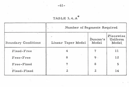
achieve a frequency root error of 5 per cent or less in the first

normal mode three increments of model (a) or (b) and eleven

incre-ments of model (d} are required.

In summary, it has been shown that models (a) and (b} give

consistent results when used to approximate the uniform system.

The errors in the non-dimensional frequency roots for these two

models decrease as l/Nz for large N. Models (c) and (d) are less

consistent in that for some boundary conditions their frequency root

errors decrease as l /N for large N; henc~, model (d} has not, in

general, shown any improvement over model (c). When considering

the higher modes two additional trends are apparent (see Figs. 3. 3. 4

and 3. 3. 5). First, the overall error level increases as expected

with higher modes for all models; and, second, the advantage of

models (a) and (b) with respect to model (c) decreases in higher

modes. The fact that the differ.ences between these models decreases for higher modes is n6t surprising, since the higher modes are less

sensitive to boundary conditions which is the main difference between

model (a) or (b) and model (c). Model (b) is slig.htly more efficient than model (a) because it achieves the same accuracy in frequency

roots with one less mass, which in turn means that the number of

differential equations is, in general, one less when using model (b).

3. 4 Linear Taper Model

Exact solutions for .non-uniform one dimensional systems

\ .

described by exact transmission matrices (see Section 3. 2). Systems which are not susceptible to exact solution can be treated in several alternative ways. A commonly recommended approach [ 1 O] is to use a piecewise uniform segment representation as shown in Fig. (3. 4. I)

A second approach, which should obviously be better, is to approxi-mate each segment by some best fit non-uniform segment for which the exact transmission matrix is known. Approximate transmission matrices can also be obtained more directly as discussed in Chapter V. A third approach is to subdivid,e the continuous system into N segments and then represent each of these segments by lumped

para-meters. In this section the lumped parameter approach will be of primary concern.

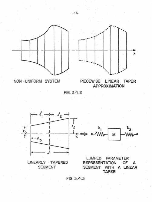
The standard way of representing the N non-uniform seg-ments by lumped parameters is to base the parameters on some mean or average uniform section for that particular segment, which is a further approximation to the £i rst case mentioned above, (see

Fig. (3. 4. 1). Duncan [ 3] derived a general error law for a particular model, which is similar to the model in Fig. (3. 4. 3)except .f. always

1

equals _{.R.. '}

2 that is used with equal segment lengths to approximate linear non-uniform systems. The goal here is to investigate the lumped parameter representation of a non-uniform segment in a more general manner in an attempt to improve upon Duncan's model and to determine if other models are more appropriate. The work

From the investigation of the uniform system, model (b) and ·model (a) of Fig.(3. 3. l)were found to be about equivalent with model

(b) being slightly more efficient; therefore, a model similar to model (b) will be employed in this sectio.n. When considering how to improve the standard lumped parameter approximation based upon uniform equivalent segments' a natural extension would be to use variable segments of prescribed variation for which simple and accurate

lumped parameters are known. For example, in one dimensional non-uniform systems where cross sections are circular the variable. radius

could be best fitted on a piecewise basis with segments that have a linearly varying radius. Once a general segment with a linearly varying radius is well approximated in terms of lumped parameters, this model could_ be applied just as the uniform segments are used and improved results would be anticipated. Figure (3. 4. 2) indicates how the piecewise linear approximation can be employed geometrically for the case of non-uniform, circular cross sectional systems. For con-venience the following development treats specifically circular cross sectional systems, but it will be emphasized later that the results apply to much more general systems.

Figure (3. 4. 3) shows ho:w a linearly tapered increment will be represented by a spring..:mass-spring model. This lumped parameter. model is essentially the same as model (b), but for the non-uniform segment the springs. are not equal; k and k represent the stiffness

l 2

of the portions of length P. and P.

NON

-

UNIFORM

SYSTEM

...

...

..

x

--~

...

....

...

...

' '

'

--

,.,

,

.

,

PIECEWISE

LINEAR TAPER

APPROXIMATION

FIG.

3.4.2

LINEARLY

·

TAPE RED

SEG

MENT

M

LUMPED

PARAMETER

REPRESENTATION

OF

A

SEGMENT

WI

TH A LINEAR

TAPER

1

-

Mwz. -Mwz.

--ic--z.

[L]

= (3.4.1)

1

+

1 Mwz. 1 Mwz.

k

k

k k

-

~

l z. l z. l

It will be shown that the L term and the first part of L ,

lZ. . Z.l

(l/k

+

l/k ), are fixed for any given increment.· The L and L

l z. . 11 z. z.

terms· are functions of 1. and /.. , however, and they can be adjusted

l z.

by the choice of these lengths. To define a criterion for choosing 1.

l

and i.

2 the lumped parameter matrix will be compared and adjusted

to approximate the exact transmission matrix for a continuous linearly

tapered segment.

Several types of tapered sys'(:ems commonly encountered in practical vibration problems can be included in the two following groups:

Group I: Cross sectional area which varies quadratically with the spatial variable.

A common example is the solid circular er.ass section with a linearly varying radius. Another is the solid rectangular cross section where height and width both vary linearly.

cross sections 'where radius varies

linearly, and solid or thin wall

rectangular cross sections where

one lateral dimension remains

constant and the other varies

linearly.

Recalling that the area function was given in Section 3. 2 as:

s;

)

Zp-1 A(x) = A

0 { 1

+

A.

it can be observed that Group l is characterized by p

=

1. 5 and

Group II by p

=

1. 0 where the definition of

s

was given as:

where:

Ai. = area at the output end of a segment

A =area at the endput end of a segment. 0

As mentioned above the following development is specifically for

circular cross sectional systems, but with the above definition of

s

there is no loss of generality and the results apply equally well to all

other systems belonging to Groups I or II.. The name erlinear taper

model" comes only from the geometrical fact that the radius does

vary linearly for circular cross sectional systems of the two groups

Group I is defined by p = 3/2; therefore, the exact

transmis-sion matrix can be obtained from Case II in Section 3, 2. Using the

following relationships:

J/

(y) = -·

r;y

siny

.1.2

VTiY

- cosy]

and the T.. expressions from Case II, the transmission matrix terms

lJ

for the cont.inuous, linearly tapered element for Group I can be writ-ten in terms of trigonometric functions as:

T

11

(1) _{= -}

f (

_{- -}sin f3

+

_cos f3)

g f (3 (3.4.2)

T (1) _{= - {}

f)

_z

0 ( (3) {sin f3

+

sin f3

+

Q:fil

_{cos f3)}

12 _{(fg) (32} fg (3. 4. 3)

T

21

(£)

={~)~o(~)

(3.4.4)

T (1) = -₍ g} ( cos f3 - - -sin f3 )

22 f

gf3

(3. 4. 5)

The transmission matrix which describes Group II, p = 1, is

obtained from Case I in Section 3. 2. The terms for this matrix

remain in Bessel function form.

T (£) = f3{Y (gf3)J (ff3)-Y (ff3)J (gf3)}

T (£) = z

(_g_

2 ) {3

2 _{{Y (f f3}J (g [3)- Y (g f3}J (ff3)}}

12 0 Tr 1 l 1 1 (3.4.7)

1 . ( f )

T (£)

= - -

-,-

{Y (f[3}J (gf3)-Y (g[3}J (f[3)}

· Zl Z t:.Tr 0 O O 0

0 .

(3.4.8)

T (,e) :::

(

1-2 ) f3{Y (ff3}J (gB)-Y (gf3)J (ff3)}

2Z Tr 0 1 1 0 (3.4.9)

Equations (3. 4. 2) through (3. 4. 9) must be expanded in series form to be compared to the matrix elements in expression (3.4.1). For the first group the trigonometric series can be used which

im-mediately gives;

T (1)

=

l..;(3z [ (£+3)]

+

0((34)

11 . 6(1 +~) (3.4. 10)

A E

T . (£) - - ~ {1+£+£2 /3}[32 + 0((34)

12 x. (3.4.11)

T

(£)

Zl (3.4.12)

T (1) = 1 -132 [ 2£

+

3]

+

O( (34 )

. Z2

- r

(3.4.13)

To expand the second group for lower order terms in

f3

is somewhat more difficult because of the behavior of Y ( 13). For small

0 2

arguments Y ((3) "' - £n(l3); therefore, Y ({3) _,. oo as

f3-+

0 and

0 Tr 0

Y (13) . can not be expanded directly in a power series of the form: 0

a + a x + a x2 + . . . • . . . + a xn

o 1 z n

The approach used to obtain a converging power series, valid for small 13, is to expand the T .. functions directly in a Maclaurin 's

lJ

that possesses finite derivatives. Applying the Maclaurin series:

I

f32

11

T .. {f3)

=

T .. (o) + f3T .. _{(o) + -21. T} .. {o) + . • .

+

lJ

lJ

lJ

lJ

and using l 'Hospital's rule to evaluate indeterminate forms gives:

Tu (1)

=

1

+

f3~

[ f.z2_gz

+

fz .ln{g/f)]

+

O{f34)

T"

(1)

=

E; 0 [ (

~'

l

£'

?'

]

+

0(

~·)

Tz1{1) =

A:E

f R.n(g/f) [1 -( f3;) fz+f z ] + 0(13'1)

T

22 (1)

=

1 -

~~

[ £'

~

g'

+

g

2

.!n(g/f)]

+

₀₍₍₃₄₎

(3.4.14)

(3. 4.15)

(3.4.16)

(3.4.17)

To check the validity of the series expansions in Eq. (3. 4. 1 O) through (3. 4. 17) the condition that

g

-+ 0, which is the uniform rod in the limit, can be imposed. Completing this for both groups above gives expressions which agree with the lower order terms in the series for the · E.. elements which were given in Section 3. 2. 1.

lJ

.

As mentioned earlier the' L term and the first part of the 12

L term, (1 /le

+

1 /k ), from expression (3. 4. 1) are fixed for any

21 1

z

given increment. This can be illustrated by using the appropriate .:r:elationships for M and w which shows that the lower order ·terms

inEqs. (3. 4.11) and (3.4.15) are always identical to ·

L .

Likewise, 12

by using the appropriate k and k expressions from Appendix C,

1

z

.

it can be shown that the order unity term in Eqs ~ (3. 4. 12) and

(3. 4. 16) is always equal to (1 /k

+

1 /k ) . The two remaining terms

which can be used to define the subdivision of a segment are L and

11

L The choice of 1. and 1. is based upon minimizing the

dif-zz l z

ference between the lower order terms in T and T and those in·

. 11

z

z

respectively. · Proceeding in this expressions for L and L

11 22.

manner gives:

11

=

1. ₁

Ii.

and 1. _l

+

1. _z

=

1.

For Group I:

Therefore,

L =

1-11

L = 1

-zz.

A E kl ::: (1+£11)

-T-:-1

A E

k

2

=

(1

+g) ( 1

+£

11)

-l--z

A E

Mwz. =

--f-:-

{l

+

g

+

£

2/3}(3z

Mwz.

1 - ( 1-:Q) (1+;+gz/3)(32

l C

= (1 +£) (l +£11)

2

Mw2

1 - 11 {1+;+gz /3}132

l <

= ( 1+g11)

Consequently, for E and E (where E •• = T .. - L .. ):

11

zz.

lJ lJ lJ

Then setting L and L

11 zz

£+3

1

z

6(1+~)

(3

E •.

=

0 to equate the coefficient of the O( (32) term in

lJ .

to that in T and T · respectively, ·gives. the follow- .

11

zz

For Group II:

k

l

EA

·O k2 =

-1.--2

2£+3 11r ~ 3(g+2)

A E

Mw2

=

+

(1+£/2}132

(3.4.18)

Setting E and E equal t.o zero as before gives an expression,

. 11 . 2 2

which is the same in both cases, for 11 II"

. (3. 4. 19} where:

b

=

2( 1 +£)2

c

=

g(2+g)

a

=

2£(2+£)

A check on both 11