IMPACT OF URBAN AGRICULTURE ON HOUSEHOLD INCOME IN
ZAMBIA: AN ECONOMIC ANALYSIS
Mavis Mupetaa
Elias Kuntashulab
Thomson Kalindac
a Graduate Student; Department of Agriculture Economics and Extension, School of Agriculture Science, University of Zambia, Lusaka, Zambia b Senior Lecturer; Department of Agriculture Economics and Extension, School of Agricultural Science, University of Zambia, Lusaka, Zambia c Associate Professor; Department of Agricultural Economics and
Extension, School of Agricultural Sciences, University of Zambia, Lusaka, Zambia
mavismupeta@gmail.com(Corresponding author)
ARTICLEHISTORY:
Received: 16-Mar-2020 Accepted: 27-May-2020 OnlineAvailable: 17-Jul-2020
Keywords:
Average treatment effect, Impact,
Poverty,
Propensity score matching, Urban agriculture
ABSTRACT
The study aimed to empirically determine the impact of urban agriculture on household income in Zambia. The analysis was based on the 2007/2008 Urban Consumption/ Expenditure secondary data collected in Kitwe and Lusaka districts, with a total sample size of 2,682 urban households. The propensity score matching approach is used to estimate the impact of urban agriculture on household income since the method takes into account the systematic differences in socio-economic characteristics between the urban agriculture practicing and non-practicing households by matching from both groups with similar characteristics. Results indicate that urban agriculture has a significant positive effect on household income. The income of households that practiced urban agriculture increased by 13.7% to 19.1%. It implies that urban agriculture has the potential to improve household livelihood through enhanced income.
\
Contribution/ Originality
This paper may be the first to apply the Propensity score matching method in the research area of urban agriculture in Zambia. The propensity score matching method was used to obtain reliable estimates of the impact of urban agriculture on household income. It helps eliminate the problem of “self- selection” bias.
DOI:10.18488/journal.ajard.2020.102.550.562 ISSN(P):2304-1455/ ISSN(E): 2224-4433
How to cite: Mavis Mupeta, Elias Kuntashula and Thomson Kalinda (2020). Impact of urban agriculture on household income in Zambia: An economic analysis. AsianJournal ofAgriculture andRuralDevelopment,10(2), 550-562.
©2020AsianEconomicandSocialSociety.Allrightsreserved.
Asian
Journal
of
Agriculture
and
Rural
Development
Volume10,Issue2(2020): 550-5621.
INTRODUCTION
Food insecurity and the high prevalence of poverty are among the most significant challenges affecting development in Sub-Saharan Africa (SSA) today (FAO, 2016; UN-HABITAT, 2010). It is estimated that about 42% of the Sub-Saharan African population live in poverty (Alkire et al., 2018). Zambia is among Southern African countries with high poverty levels. About 60% of the Zambian population lives in poverty (World Bank, 2019). Achieving poverty reduction has been a developmental agenda of the country (Woodbridge, 2015).
Agriculture has been recognized as an important sector with the potential of alleviating poverty and ensuring food security. It has become the economic backbone of the country, contributing approximately 20% to Gross Domestic Product (GDP) in 2008. In 2018, the sector’s contribution to Gross Domestic Product (GDP) declined to about 2.6% (Plecher, 2018; World Bank, 2019). Agriculture is the main activity among rural households accounting for the employment of about 80% of the rural population (CSO, 2012). Henceforth, the government, in collaboration with other stakeholders, has developed sustainable agriculture technologies to improve food productivity and security. The focus has been in rural areas where the activity is predominant, and poverty levels are high.
However, the current global rapid rate of urbanization has posed a threat to food security in urban areas of Zambia and Sub-Saharan Africa (SSA) at large (Crush and Frayne, 2010; Stewart et al., 2013). In 2000, 38% of Africans lived in urban areas, and the figure is projected to increase to 55% by 2030 (UNHABITAT, 2010). Zambia has been reported to be the third most highly urbanized country in SSA. According to reports, about 40% of its total population is estimated to live in urban areas (World Bank, 2011; CSO, 2012). Urbanization or urban population growth in Zambia is a result of rural-urban migration, natural population growth, economic recessions, and structural adjustment programmes (Masvaure, 2013; Hampwaye, 2010).
The increased urban population has been associated with high food prices, among others (Padgham et al., 2015). Urban households mainly access their food through purchases, unlike rural households who consume from their produce (Badami and Ramanculty, 2015). Food alone accounts for 50-80% of their disposable income (Masvaure, 2013; CSO, 2012). An increase in food prices reduces their purchasing power, thus threatening food security. Although agriculture is typically thought of as a predominantly rural activity, the majority of urban households, especially in SSA, have resorted to farming as a coping strategy to mitigate hunger. It is reported that about 40% of the population in African cities are involved in urban agriculture (FAO, 2012).
Generally, there exists a consensus among many scholars that urban agriculture does improve household food security through improved nutrition and increased income (Badami and Ramankutty, 2015; Warren et al., 2015; Masvaure, 2013; Salcu and Attah, 2012; Kutiwa et al., 2010; Smit et al., 2001; Armar, 2000; Nugent, 2000; Mbiba, 1994; Mbiba, 1998; Maxwell, 1994). It was also observed that a number of studies (for example, Masvaure, 2013; Salcu and Attah 2012;
Kutiwa et al., 2010; Zezza and Tasciotti, 2010) had used regression analysis to determine the impact of urban agriculture on household income. Empirical research by Masvaure (2013) indicated that urban agriculture provides a cheaper source of food for urban farmers through the consumption of their own produce. Access to food from urban agriculture releases extra money for other expenses like transport, health, education, water, and electricity.
Kutiwa et al. (2010) used a simple regression model to estimate the effect of urban agricultural income on total household income. The results showed that total farm income has no significant impact on total household income. A limitation of such an analysis is the problem of endogeneity. Other factors, such as income from non-farm activities, could play a role in influencing the level of income from urban agriculture.
Zezza and Tasciotti (2010) studied the impact of urban agriculture on income with a focus on the income share from urban agriculture. The study found that the percentage of urban households that earn income from agriculture varied from 11% in Indonesia to about 70% in Vietnam and Nicaragua. Income from urban agriculture as a share of total income ranged from 1% to 27%.
However, the major drawback of these studies is that analysis was done by just computing and directly comparing the outcome incomes of participants and non-participants without considering the differences in their household characteristics. This might have resulted in inconsistent and biased conclusions (Heckman et al., 1998). Against this background, this study employed the Propensity Score Matching (PSM) methods to estimate the Average Treatment Effect on the Treated (ATT). The estimated ATT was used to measure the impact of urban agriculture on household income. In Zambia, none of the previous studies has applied the PSM methods to measure the impact of urban agriculture on household income.
Another significant contribution of this paper is that unlike other studies that used household income as the outcome variable, this study used household total expenditure as a proxy for household income. The disadvantage of using income is that some households tend to give distorted figures of their income, which in most cases, is less than their actual income. In such cases, data collected on income tends to be unreliable, and results may not give a true reflection of the impact of urban agriculture on household income.
Therefore, the main objective of this study was to give more precise estimates of the impact of urban agriculture on household income in Zambia.
2. MATERIALS AND METHODS
2.1. The data
This study used secondary data from the 2007/2008 urban food consumption/expenditure survey conducted by the Central Statistical Organization (CSO) and Indaba Agricultural Policy Research Institute (IAPRI) in Lusaka, Kitwe, Mansa, and Kasama districts of Zambia. The total sample size was 4,800 households, but this study only focused on data captured from two districts, namely Lusaka and Kitwe districts, with a sample size of 2,682 households. Lusaka and Kitwe districts were purposively selected in this study because the study narrowed its focus to urban agriculture in the cities. Lusaka and Kitwe are cosmopolitan cities, Lusaka being the capital city of Zambia and Kitwe, is the largest city on the Copperbelt Province while Kasama and Mansa are more of rural districts. The Urban Food Consumption/Expenditure data was used in this study because it had a component of urban agriculture that was relevant to this study.
2.2. Econometric model
affected by the treatment, potential outcomes Y are independent of treatment assignment D specified by:
Y0 , Y1 Di/Xi.It assumes that assignment to treatment is independent of the outcomes, conditional on the covariates. The second is the common support or overlap condition, which implies that the probability of assignment to a treatment is positive but less than one. It is specified by:
1/
10P Di Xi .
It implies that treatment observations have comparison observations “nearby” in the propensity score distribution. If there is little or no overlap in the distributions of the estimated propensity scores in the treatment groups, the estimated ATT would be invalid. It is more convenient to use propensity scores than covariates to match treated and non-treated units. Propensity scores eliminate dimensionality complications in a large set of covariates. The outcome of participants and non-participants with similar propensity scores can then be compared to obtain the treatment effect. The propensity score is defined as the conditional probability that a unit in the combined sample of treated and untreated units receives the treatment, given a set of pre-treatment characteristics (Heckman et al., 1998; Rosenbaum and Rubin, 1983). It is specified as:
Xi
Di Xi
P Pr 1/ .
Applying the PSM method, a logistic regression model was used to estimate propensity scores. The general principle is to include only variables that influence the treatment status and the outcome variable (Smith and Todd, 2005) simultaneously. Variables that were included in the PSM model were: the gender of the household head, marital status of the household head, the size of the household, age of the household head, the highest level of education of the household head, city of residence of the household, number of adult members of the house, the household’s main source of livelihood, class of residence, the expected market price of maize, the expected market price of groundnuts, expected market price of rape. A balancing test was done to check the balancing properties of the propensity scores to obtain estimates that statistically balance the covariates between treated and control units. Urban agriculture participants and non-participants with similar values of propensity scores were matched. Matching was implemented using the Nearest Neighbor (NN) without replacement, Kernel, and Radius matching algorithms to ensure the robustness of estimates (Caliendo and Kopeinig, 2008).
The Average Treatment effect on the Treated (ATT) was computed using the general model:
X i
i
i
i
i
i
i
pPSM
ATT E D EY D P X EY D P X
T
i / 1 1 / 1, 0 / 0,
Where:
T
ATTPSM=Average Treatment on the Treated;
Y
iD
iP
X
i
E
1
/
1
,
=observed change in income of urban agriculture participants;
Y
iD
iP
X
i
E
0
/
0
,
= observed change in income of urban agriculture non- participants;
XiP =Conditional probability of participation in urban agriculture given X
3. RESULTS AND DISCUSSION
3.1. Descriptive analysis
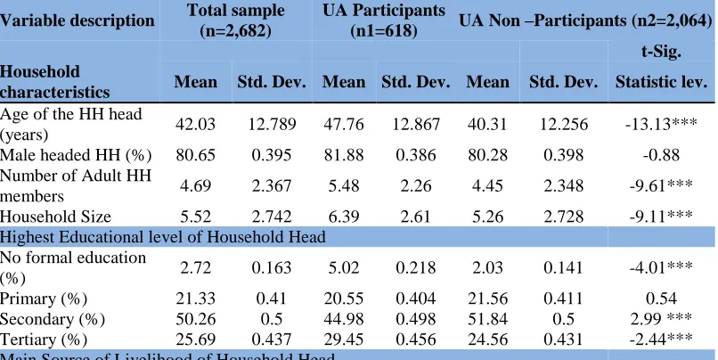
A summary of the socio-economic characteristics of the sampled households used in this study is shown in Table 1. Out of the 2,682 households that were included in this study sample, only 23% (618) of the households were practicing farming. Comparably, results further show statistically significant differences in the households’ characteristics between urban agriculture participants and non-participants. The majority of the sampled households were male-headed (80.6%). The age of the respondents ranged from 19 to 90 years. The average age of the household head was 42 years. The average age of the household head for participants and non-participants was 48 years and 40 years, respectively. Notably, older household heads were more likely to engage in farming.
Most of the sampled household heads were monogamously married (70.5%), 10.1% were never married before, 0.7% were in polygamous marriages, 5% were divorced, 12.2% were widowed, 1.5% were separated, and only 0.07% were cohabiting. About 76.4% of urban agriculture household heads were married, while about 69.6% of non-urban agriculture household heads were married.
Results indicate that urban agriculture participants are more likely to be married compared to non-participants. Among the unmarried respondents, urban agriculture households tended to have a higher proportion of widowed heads (14.6%) than non-agriculture households (11.4%). It suggests that widows were more likely to resort to urban agriculture to fend for themselves and their families.
In terms of the distribution of education, 97.3% of the respondents had attended formal education. Of those respondents who attended school, 21.3% attended only primary education while more than half (50.3%) managed to attain a secondary level of education. In addition, a relatively high percentage (25.7%) of the respondents managed to attain a tertiary level of education. This could be attributed to the increase in the number of tertiary education facilities in most parts of urban Zambia. Similarly, urban agriculture household heads were more learned (29.4% had reached tertiary education) than non-agriculture household heads (24.6% had reached tertiary education). From the total sample, about 50% of the respondents were located in Kitwe, while the others were located in the Lusaka district.
Table 1: Descriptive statistics of variables
Variable description Total sample (n=2,682)
UA Participants
(n1=618) UA Non –Participants (n2=2,064) t-Sig. Household
characteristics Mean Std. Dev. Mean Std. Dev. Mean Std. Dev. Statistic lev. Age of the HH head
(years) 42.03 12.789 47.76 12.867 40.31 12.256 -13.13*** Male headed HH (%) 80.65 0.395 81.88 0.386 80.28 0.398 -0.88 Number of Adult HH
members 4.69 2.367 5.48 2.26 4.45 2.348 -9.61***
Household Size 5.52 2.742 6.39 2.61 5.26 2.728 -9.11***
Highest Educational level of Household Head No formal education
(%) 2.72 0.163 5.02 0.218 2.03 0.141 -4.01***
Primary (%) 21.33 0.41 20.55 0.404 21.56 0.411 0.54
Secondary (%) 50.26 0.5 44.98 0.498 51.84 0.5 2.99 ***
Formal business (%) 6.75 0.251 4.85 0.215 7.32 0.26 2.23 Informal business
(%) 23.01 0.421 18.12 0.386 24.47 0.43 -1.91
Farming (%) 3.28 0.178 7.61 0.265 1.98 0.14 -4.52
Other wages (%) 6.86 0.253 5.83 0.234 7.17 0.258 0.71
Salaried employment
(%) 52.13 0.5 50.97 0.5 52.47 0.5 0.65
Location of Residence of Household Low-cost residential
(%) 72.56 0.446 65.7 0.475 74.61 0.435 4.37***
Medium cost
residential (%) 10.14 0.302 9.22 0.29 10.42 0.306 0.86
High cost residential
(%) 17.3 0.378 25.08 0.434 14.97 0.357 -5.86***
Marital Status of Household Head Married Head of HH
(%)
Never married HH
head (%) 10.14 0.302 4.53 0.208 11.82 0.323 5.29***
Monogamously
married (%) 70.47 0.456 75.73 0.429 68.9 0.463 -3.27***
Polygamous married
(%) 0.71 0.084 0.65 0.08 0.73 0.085 0.21
Divorced (%) 5 0.218 3.56 0.185 5.43 0.227 1.87*
Widowed (%) 12.16 0.327 14.72 0.355 11.39 0.318 -2.23**
Separated (%) 1.45 0.12 0.81 0.09 1.65 0.127 1.53
Cohabiting (%) 0.07 0.027 0 0 0.1 0.031 0.77
City of Residence of Household Head HH located in Kitwe
(%) 50.41 0.5 66.83 0.471 45.49 0.498 -9.46***
HH located in Lusaka
(%) 49.59 0.5 33.17 0.471 54.51 0.498 9.46***
HH Monthly
Expenditure (K) 1815.85 1876.14 2222.25 2398.453 1694.17 1670.2 -6.18*** Note: Unequal-variance t test: *, **, and *** represents 10%, 5%, and 1% level of significance
This means that both cities had an almost equal representation of the total sample size. However, a significantly larger proportion of households of Kitwe (66.8%) were adopters of urban agriculture compared to Lusaka (33.2%).
Results further indicate that 72.6% of the total respondents were from the low-cost residential areas, 10.1% were from the medium-cost residential regions, and 17.3% were from the high-cost residential regions, as highlighted in Table 1. These results suggest that majority of the households included in the study sample were from the low-cost (low income) residential areas. A significant difference was noted in terms of the households’ residential area between participants and non-participants. Contrary to the belief that low-cost residential households are more likely to engage in farming, the study results show that households from the high cost (25.1% participants vs. 15% non-participants) areas were relatively more likely to engage in farming than households from the low-cost area.
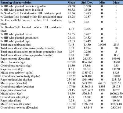
3.1.1. Household farming characteristics
and rape (vegetable). Households who grew one or more of these crops within the boundaries of their town of residence were captured as farming households. The decision to limit urban agriculture to maize, groundnuts, and rape production was guided by the significant proportion of households who engaged in the production of these crops as well as the average area of production relative to other crops. The other crops that were grown by the sampled households included cabbage, spinach, tomato, onion, okra, sorghum, millet, soybeans, mixed beans, sweet potatoes, cassava, pumpkins, and cowpeas.
Results show that the total number of households practicing urban agriculture was 618 households. The participating farming households grew their crops either in a garden or in a field, at around 50% apiece. Results also indicate that the fields or gardens used for crop production were located in four (4) different residential areas; either within the households’ residential plot, within the households’ residential area but outside its residential plot, within the households’ town of residence but away from its residential area, or outside the households’ town of residence.
Table 2: Summary statistics of farm characteristics of urban farming households
Farming characteristics Mean Std. Dev. Min Max
% HH who planted crops in a garden 49.68 0.500 0 1
% HH who planted crops in a field 50.32 0.500 0 1
% Garden/field located inside HH residential plot 41.26 0.493 0 1 % Garden/field located within HH residential area 18.28 0.387 0 1 % Garden/field located within HH residential
town 36.09 0.481 0 1
% Garden/field located outside HH residential
town 4.37 0.205 0 1
% HH who planted maize 61.65 0.487 0 1
% HH who planted groundnuts 28.48 0.452 0 1
% HH who planted rape 27.83 0.449 0 1
Total area cultivated (ha) 0.45 1.480 0.0005 25.5
Total area allocated to maize production (ha) 0.37 1.284 0 20 Total area allocated to groundnuts production (ha) 0.07 0.266 0 5 Total area allocated to rape production (ha) 0.01 0.031 0 0.5
Rape revenue (Kwacha) 1.93 26.430 0 599.91
Maize harvests (kg) 207.08 886.563 0 11500
Groundnuts harvests (kg) 11.50 57.864 0 950
Rape harvests (kg) 1.51 10.018 0 139.91
Maize productivity (kg/ha) 544.49 1385.471 0 8625
Groundnuts productivity (kg/ha) 132.29 688.483 0 10000
Rape productivity (kg/ha) 234.86 1044.980 0 233175
Maize price (kwacha) 13.08 593.292 764.70 3823.50
Groundnuts price (kwacha) 107.46 5136.348 5593 28173
Rape price (kwacha) 29.15 1421.687 1390 8575
Maize sales (Kgs) 54.59 570.547 0 100062.50
Groundnuts sales (Kgs) 1.29 12.883 0 10062.50
Rape sales (Kgs) 0.38 4.149 0 69.96
Maize revenue (Kwacha) 101.70 1326.180 0 30779.18
Groundnuts revenue (Kwacha) 19.08 185.145 0 2830.96
Note: n = 618
gardens were found inside the households’ residential area. Only a small proportion of households’ gardens and fields were located outside the town of residence (4.4%). However, this study was interested only in urban farming households with gardens and fields found within the limits of the boundaries of the town of household residence (within Lusaka and Kitwe cities). It means the households with fields and gardens along the periphery of the city of residence or outside Lusaka and Kitwe cities were not included in the study. These results show that urban farmers have a challenge of access to land for crop production. Most of the households use land within the confinement of their compounds for farming.
Around 61.7 %, 28.5%, and 27.8 % were involved in maize, groundnuts, and rape production, respectively. These results indicate that maize was highly grown among the respondent households. This may be attributed to the crop’s significance as a staple food of the country. The average household farm area under cultivation was only 0.45 hectares (Table 2). A significantly larger portion of this land was allocated to maize (0.37 ha) production. Only 0.07 ha was allocated to the production of groundnuts, and a lesser amount (0.01 ha) was used for growing rape. A possible explanation is that in this study, all the rape produced by the farming households was grown in gardens. Most of the gardens were located in the backyards of the households’ residential plots with limited available space for gardening.
Results also revealed that among urban agriculture participants, the average crop productivity for maize, groundnuts, and rape was 544.5kg/ha, 132.3kg/ha, and 234.9kg/ha compared to the national average crop yield of maize and groundnuts which are about 1.5mt/ha and 0.68mt/ha respectively. On average, a total of 201.1 kilograms of maize, 11.5 kilograms of groundnuts, and 1.5 kilograms of rape were harvested. Of these harvests, only 54.6 kilograms of maize was sold, indicating a proportion of 21.2 % sales of the total harvests. 1.3 kilograms of groundnuts (11.2 %) were sold, and 0.38 kilograms of rape (25.1%) were sold. This means that major portions of crops harvested were retained for home consumption. These results suggest that most of the urban farmers are subsistence farmers. Crops are mainly grown for household food consumption, nutrition, and food security.
3.2. Empirical findings
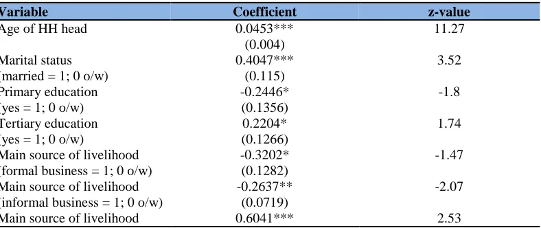
The propensity to participate in urban agriculture was positively influenced by the age of the household head, the household head being married, and the household head having attained tertiary level of education; having farming as the main source of livelihood and being a resident of Kitwe. However, being a resident of a low-cost area, having attained a primary level of education, and having formal and informal businesses as the main source of livelihood negatively influenced the propensity to practice urban agriculture.
Table 3: Propensity score estimates of urban agriculture
Variable Coefficient z-value
Age of HH head 0.0453*** 11.27
(0.004)
Marital status 0.4047*** 3.52
(married = 1; 0 o/w) (0.115)
Primary education -0.2446* -1.8
(yes = 1; 0 o/w) (0.1356)
Tertiary education 0.2204* 1.74
(yes = 1; 0 o/w) (0.1266)
Main source of livelihood -0.3202* -1.47
(formal business = 1; 0 o/w) (0.1282)
Main source of livelihood -0.2637** -2.07
(informal business = 1; 0 o/w) (0.0719)
(farming = 1; 0 o/w) (0.2389)
Category of residence -0.4835** -4.13
(low-cost = 1; 0 o/w) (0.1169)
Town of residence 0.8263*** 8.09
(Kitwe = 1; 0 o/w) (0.1021)
Constant -3.5793 -14.96
Pseudo R2 = 0.10 Prob>Chi2
*, **, and *** represents 10%, 5%, and 1% level of significance respectively
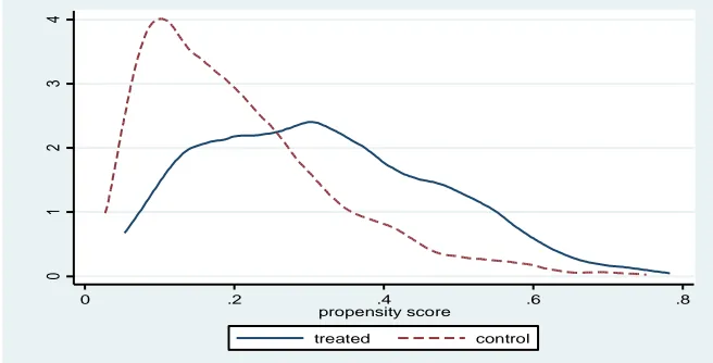
3.2.1. Region of common support
The condition of common support was selected and satisfied in the region of [0.053_0.783]. Observations whose propensity scores lay outside the region of common support were discarded from the estimation of the impact of urban agriculture on household income (see Figure 1). Out of 2, 682 observations, 2, 603 observations were matched, meaning that 79 observations were discarded. These were households with propensity score values below 0.053 and above 0.783. The optimal number of blocks used to define the region of common support was eight blocks. This number of blocks ensured that the mean propensity score was not different for treated and controls in each block. Below is a graphical presentation of the region of overlap or common support.
Figure 1: Area of common support for the treatment and control groups
3.2.2. Balancing tests of propensity scores and covariates - t-test
The t-test was applied by comparing the statistical significance of the mean differences of the covariates between the treated group and the untreated group both before and after matching. According to this test, the balancing property of the matching methods is satisfied if the mean differences of the covariates between the treated group and the untreated group are statistically insignificant after matching. Several variables showed statistically significant differences before matching. After matching, the differences were minimal and statistically insignificant, suggesting that the balancing property was satisfied (Table 4).
Table 4: Balancing tests of propensity scores and covariates (t-tests and standardized % bias)
Variable Sample Participants
Non-participants % bias t p>t
Age Unmatched 47.775 40.311
Matched 47.775 47.651 1.0 0.16 0.870
Married Unmatched 0.764 0.696
0
1
2
3
4
kd
en
si
ty
lo
gi
t1
0 .2 .4 .6 .8
propensity score
Matched 0.764 0.755 1.9 0.35 0.723
Primary Unmatched 0.206 0.216
Matched 0.206 0.204 0.3 0.05 0.957
Tertiary Unmatched 0.294 0.246
Matched 0.295 0.299 -0.9 -0.16 0.874
Formal Unmatched 0.049 0.07
Business Matched 0.049 0.046 0.9 0.17 0.864
Informal Unmatched 0.181 0.245
Business Matched 0.181 0.188 -1.5 -0.29 0.775
Farming Unmatched 0.076 0.020
Matched 0.076 0.066 4.8 0.70 0.483
low-cost Unmatched 0.657 0.746
Matched 0.657 0.659 -0.5 -0.08 0.933
Kitwe Unmatched 0.668 0.455
Matched 0.668 0.658 2.0 0.36 0.715
*, **, and *** represents 10%, 5%, and 1% level of significance respectively 3.2.3. Impact of urban agriculture on household income
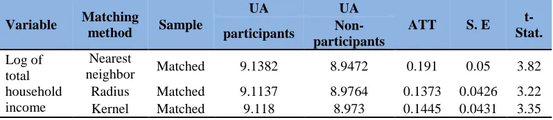
Results on the impact of urban agriculture on household income from the three matching algorithms used are shown in Table 5. The nearest neighbor matching methods showed that urban agriculture had a positive and significant impact on household income. Engaging in urban agriculture increased household income by 19.1%. Likewise, radius matching methods indicated that urban agriculture had a positive and significant impact on household income. Practicing in urban agriculture increased household income by 13.7%. Kernel matching methods further confirmed the impact of urban agriculture on household income. According to the kernel matching method, urban agriculture increased household income by 14.5%. All the three matching methods used were consistent on the estimated impact of urban agriculture on household income with a very narrow variation in the estimates. It can be observed and concluded from the results that controlling for observable characteristics, participation in urban agriculture would increase household income in the ranges of 13.7% to 19.1%. These results were significant at a 95% confidence level. These results are consistent with other studies such as Salcu and Attah (2012) and Zezza and Tasciotti (2010), who also concluded that urban agriculture is positively related to household income. Table 5: Expected log of total household income: treatment effects of urban agriculture
Variable Matching
method Sample
UA UA
ATT S. E
t-Stat.
participants
Non-participants Log of
total household income
Nearest
neighbor Matched 9.1382 8.9472 0.191 0.05 3.82
Radius Matched 9.1137 8.9764 0.1373 0.0426 3.22
Kernel Matched 9.118 8.973 0.1445 0.0431 3.35
explanation could be that access to land for farming is a limiting factor; hence households produce only enough for home consumption. This explanation is drawn from the fact that the majority (about 41%) of households’ fields/gardens are located within the confinements of their residential plots. Further, the mean urban household farming area is only about 0.45 hectares (Table 2), compared to about 1.5 to 2.0 hectares for small scale farmers in the rural areas of Zambia. The majority of urban households have access to land for cultivation of fewer than 0.10 hectares.
The observed additional income of households that practiced urban agriculture was from both money savings realized as a result of the households’ reduction in expenditure on food for home consumption, as well as cash income from the sale of the surplus produce. However, the increase in income from savings was more than the increase in income from the sales revenue. These results are consistent with findings by other studies such as Masvaure (2013), who found that urban agriculture provides a cheaper source of food for urban farmers through the consumption of their produce. Access to food from urban agriculture releases extra money for other foods and non-food expenses. The average revenue obtained from maize, groundnuts, and rape sales were K101.70, K19.08, and K1.93, respectively (Table 2). Furthermore, it was observed that compared to the other crops, rape was the most sold crop. This could be because of the availability of a ready market for the crop.
These results imply that urban agriculture has the potential to reduce poverty, enhance the standard of living, and improve household food security through increased household income and improved nutrition.
4. CONCLUSIONS AND RECOMMENDATIONS
Results confirm the potential of urban agriculture to contribute to increased household income. Farming households showed higher incomes than non-farming households with similar socio-economic characteristics. Increased income is through savings on food purchases and selling of produce. These results are consistent with other reviewed studies. It is recommended that the Government of Zambia should create an enabling environment for urban agriculture by integrating it into the Agricultural Policy. Adequate research on the extent of the practice, constraints, opportunities, and potential benefits of urban agriculture is recommended. Urban households should be encouraged to consider adopting urban agriculture as a source of food, diversified nutrition, and income.
Funding: This study did not receive any specific financial support.
Competing Interests: The authors declare that they have no competing interests.
Contributors/Acknowledgement: All authors participated equally in designing and estimation of current research.
Views and opinions expressed in this study are the views and opinions of the authors, Asian Journal of Agriculture and Rural Development shall not be responsible or answerable for any loss, damage or liability, etc. caused in relation to/arising out of the use of the content.
References
Alkire, S., Kanaaratam, U., & Suppa, N. (2018). Global dimensional poverty index. OPHI Briefing No. 417, Oxford poverty and human development initiative. Oxford University.
Armar, K. M. (2000). Urban agriculture and food security, nutrition and health. In: Bakar, et al. (ed) Growing Cities, Growing Food. DSE, Feldafing, p 99-113.
Badami, M., & Ramankutty, N. (2015). Urban Agriculture and Food Security: a critique based on assessment of urban land constraints. Global Food Security, 4, 8-15. doi.org/10.1016/j.gfs.2014.10.003
doi.org/10.1007/3-540-28708-6_4
Central Statistics of Zambia (2012). Census of population and housing: national analytical report. Central Statistical Office, Lusaka.
Crush, J., & Frayne, B. (2010). Pathways to insecurity: urban food supply and access in Southern
African Cities. Urban Food Security Series No: 3. African Food Security Urban Network
(AFSUN).
FAO (2012). The first status report on urban and peri-urban horticulture in Africa: Growing green
cities in Africa. Food and Agriculture Organization of the United Nations.
FAO (2016). Africa regional overview of food and nutrition. the challenges of building resilience to
shocks and stress. Food and Agriculture Organization of the United Nations.
Hampwaye, G. (2010). Inclusive or exclusive globalization? Zambia’s economy and Asian investment. Africa Today, 56(3), 84-102.
Heckman, J., Ichimura, H., Smith, J., & Todd, P. (1998). Characterizing selection bias using experimental data. Econometrica, 66(5), 1017-1098.
Kutiwa, S., Boon, E., & Devuyst, D. (2010). Urban agriculture in low income households of Harare: an adaptive response to economic crisis. Journal of Human Ecology, 32(2), 85-96. doi.org/10.1080/09709274.2010.11906325.
Masvaure, S. (2013). Coping with food poverty in cities. The case of urban agriculture in Glen Norah Township in Harare school of community development, Faculty of humanities. Maxwell, D. G. (1994). The household logic of urban farming in Kampala. Cities feeding people:
An examination of urban agriculture in East Africa,IDRC, Ottawa, 146, 47-65.
Mbiba, B. (1994). Institutional response to uncontrolled urban cultivation in Harare: Prohibitive or accommodative? Environment and Urbanisation, 6, 188-202. doi.org/10.1177/095624789400600116.
Mbiba, B. (1998). Urban agriculture policy in Southern Africa: from theory to practice; town and
recreational planning. University of Sheffield: Paper presented at the international
conference on productive open space management. Technikon, Pretoria.
Nugent, R. (2000). The impact of urban agriculture on the household and local economies. Growing cities, growing food: urban agriculture on the policy agenda. Eurasbury, Germany: 67-97.
Padgham, J., Jabbour, J., & Dietrich, K. (2015). Managing change and building resilience: A Multi-stressor analysis of urban and peri-urban agriculture in Africa and Asia. Urban climate
system for analysis research training, USA., 12, 183-204.
Plecher, H. (2020). Share of economic sectors in GDP in Zambia 2008b to 2018. Retrieved from
https://www.statista.com.Zambia.
Rosenbaum, P. R., & Rubin, D. B. (1983). The central role of propensity score in observational studies for causal effects. Biometrika, 70, 42-55.
Salcu, E. S., & Attah, A. J. (2012). A socio-economic analysis of urban Agriculture in Nasarawa
state, Nieris. Department of agricultural Economics and Extension, Navarawa state
university.
Smit, J., Nasr, J., & Ratta, A. (2001). Benefits of urban agriculture, urban agriculture food, Jobs
and sustainable cities. The Urban Agriculture Network, Inc.
Smith, J., & Todd, P. (2005). Does matching overcome lalondes’s critiques of non-experimental estimators? Journal of Economics, 125(1-2), 305-353. doi.org/10.2139/ssrn.286297. Stewart, R., Korth, M., Langer, L., Rafferty, S., Da Silva, N., & Van Rooyen, C. (2013). What are
the impacts of urban agriculture programs in food security in low and middle-income countries. Environmental Evidence, 2(7), 1-2. doi.org/10.1186/2047-2382-2-7.
UN-HABITAT (2010). The state of African cities 2010. Governance, inequalities and urban land markets, Nairobi. United Nations Human Settlement Programme (UN_HABITAT).
https://sustainabledevelopment.un.org.
Woodbridge, M. (2015). From MDGs to SDGs: what are the sustainable development goals? ICLEI Briefing Sheet-Urban Issues, No.01 Bonn, Germany: ICLEI-Local Governments for Sustainability.
World Bank (2011). World development indicators: agriculture for development. Washington DC: World Development Indicators.
World Bank (2019). The world bank in Zambia: Overview. IBRD. IDA.
https://www.Worldbank.org.