Type of the Paper (Article)
1
Three-Dimensional Facies Analysis using
2
Object-Based Geobody Modeling: A Case Study for
3
the Farewell Formation, Maui Gas Field, Taranaki
4
Basin, New Zealand
5
AKM Eahsanul Haque1*, Md. Aminul Islam1 and Mohamed Ragab Shalaby1
6
1 Department of Physical and Geological Sciences, FoS, Universiti Brunei Darussalam, Jalan Tungku Link,
7
Gadong BE-1410, Brunei Darussalam; [email protected]
8
* Correspondence: [email protected]; Tel.: +673-7219745
9
Abstract: The early-mid Paleocene Farewell Formation is stratigraphically distributed across the
10
southern Taranaki Basin (STB) which is also encountered within the Maui Gas Field. Using
11
available 3D seismic and well log data, a challenging task to delineate the spatial distribution and
12
geobody patterns of the potential reservoir sands of the formation was performed. Object based
13
modeling coupled with sequential indicator simulation were used to analyze the spatial
14
distribution of facies configuration and a conceptual model was developed based on the outputs
15
from the structurally- modeled grids. The facies modeling followed a hierarchical object-based
16
mechanism which was set to perform with constraints like channel geometry and heterogeneity
17
within the formation. The resultant 3D geobody model showed that the distributary channels,
18
mainly braided geobodies flowed from northeast cutting through several regional normal-fault
19
systems to the southwest. Overbank facies was adhered to the fringe of the channels whereas the
20
floodplain facies was at the periphery of the model. Meandering channel-sand facies were mostly
21
observed at the center of the model flowing in a more random manner, occupying major flow
22
directions of northwest to southwest and southeast to northwest within the model.
23
Keywords: Geobody Modeling, Object-Based Facies Modeling (OBFM), Variogram Analysis,
24
Farewell Formation, Paleo-depositional Environment.
25
1. Introduction
26
The Maui Field produces gas from three main reservoirs of Paleocene to Eocene in age. Farewell
27
Formation is the deepest and the thinnest of the reservoirs of this gas field having measured drilling
28
depths ranging from 3100-3200m TVDSS [1-4]. The Farewell Formation in the Maui Gas Field
29
includes gas and condensate-saturated interval of approximately 100m thickness. The reservoir
30
interval consists of highly discontinuous fluvial sandstones and associated siltstones and shales
31
deposits as identified in the well log responses. The main reservoir sandstones are braided and
32
meandering stacked channel sand deposits that are highly lenticular, with lateral dimensions
33
ranging from few hundred to several kilometres in length [5-8]. Crevasse-splay deposits comprise a
34
relatively lower proportion of the overall sandstone volume and are generally of lower reservoir
35
quality [5].
36
Therefore, an understanding of the structure as well as the thickness, distribution and
37
connectivity of the sandstone deposits as separate geobody units are important for the well planning
38
during future development of the field. This is significant because during well planning phase,
39
500-1500m spacing between wells is often necessary to effectively deplete the reservoir given the
40
limited lateral extent of the fluvial sandstones within prospective formations like that of Farewell
41
[9-10]. Even with intensive development of the Farewell reservoir with spacing of 1-2 km for future
42
43
Figure.1. Maui Gas Field and the surrounding regions of the Taranaki Basin, New Zealand (after Haque et al.
44
2016). The yellow colored compartments are two producing blocks of the Maui Gas Field. N-S elongated lines
45
are the major faults cutting through the gas field. The gas field sits on the Central Graben which is located at the
46
Southern Taranaki Basin (STB).
47
48
drillings, bottom-hole pressure tests revealed that almost all the major sand packages tested in all
49
four wells were in pressure communication showing partial pressure depletion [11-13].
50
The primary objectives of this study were (1) to interpret the primary stratigraphic framework
51
of the Farewell interval within the study area of the Maui Gas Field, (2) to characterize and model
52
lithology distribution according to the environment of deposition, (3) to explain the predicted fluvial
53
sand-bodies within the reservoir and paleo-depositional modeling of the Farewell reservoir for
54
56
Figure.2. Seismic cube of the Maui Gas Field showing well locations and 3D geomodel of the Farewell
57
Formation.
58
59
The study area is within the northern portion of the offshore Taranaki Basin (Fig.1) and includes
60
well information and 3D seismic data. The seismic survey covers an area of ~150 sq. km with average
61
grid size of the cube being 50m X 50m (Fig.2). The interval of interest for this study approximately
62
coincides with the mainly condensate/gas-productive interval at the Maui Gas Field and includes an
63
average of ~100m thick interval of the Farewell Formation.
64
65
Figure.3. Regional Structural setup of the Taranaki Basin. Grey shading represents basement (after King and
66
Thrasher 1996). The pre-Miocene configuration of the basin’s eastern margin is uncertain (Reilly et al. 2015).
67
sediment thicknesses, and incorporate paleo-bathymetry; no allowance was made for sediment de-compaction,
69
and the sections have not been structurally balanced. The original thickness of Miocene sediment is uncertain.
70
2. Geological Setup and Stratigraphy
71
The Taranaki Basin has a composite morphology resulting from diverse episodes of tectonic
72
activity [2, 14-15]. It consists of several superimposed sub-basins, depocentres, and areas of uplift,
73
that range in age from mid-Cretaceous to Recent (Fig.3). The basin’s structural development was
74
influenced by contrasting Australian-Pacific plate boundary kinematics in the Late
75
Cretaceous-Paleocene and in the Oligocene-Neogene, separated by a relatively quiescent period
76
throughout most of the Eocene [6, 16-18]. Taranaki Basin is broadly divided into Western Stable
77
Platform and the Eastern Mobile Belt [6-7, 18], and Maui Gas Field sits on the EMB. EMB in the
78
previous literatures reflects the composite architecture and evolution of the basin, involving several
79
tectonic phases of differ in age, origin and style [8, 19-20].
80
81
Figure.4. Generalized Stratigraphy of the Taranaki Basin. Farewell Formation is at the bottom of the Paleocene
82
period of the Taranaki stratigraphy (after King and Thrasher 1996). Parts of the yellow colored (dotted) sands
83
are Farewell Formation on the stratigraphic chart.
84
85
Stratigraphically Farewell Formation falls within Kapuni Group of Paleocene age (Fig.4).
86
Paleocene and Eocene deposits belong to the laterally equivalent Kapuni and Moa groups, which
87
constitute a late-rift and post-rift transgressive sequence [6, 18]. The Apart from Farewell Formation,
88
Kapuni Group also consists of Kaimiro, Mangahewa, and McKee formations. It is predominantly
89
terrestrial, including some marginal marine deposits [6-8]. A paraconformity at the top of the
90
Moa-Kapuni succession reflects waning subsidence and sediment supply, and marks the
91
culmination of this depositional phase in the latest Eocene-Early Oligocene.
92
3. Materials and Methods
98
3.1. Dataset
99
100
Figure.5. The Farewell model is identified in accordance with the 3D seismic interpretation from the Maui cube.
101
The mesh grill top and bottom (blue and yellow) are model boundaries whereas the different coloured vertical
102
pillars are the faults interpreted along the entire 3D structural grid of the Maui Gas Field. The seismic surface
103
(pink coloured) denotes the interpreted Farewell reservoir zone.
104
105
The first well of the Maui Gas Field has been drilled in 1969 and the last so far being drilled in
106
early 2000s; we have used 17 available well data for the current study from which 4 wells have
107
encountered Farewell Formation. In order to move forward for greater accuracy in delineating
108
possible geobodies, we utilized well location data along with the log data. A detailed collection of
109
conventional well log have been available for the study, namely Gamma Ray (GR), Caliper,
110
Resistivity (Shallow/Deep), Neutron, Density and Sonic. A set of formation tops of the Farewell
111
Formation for all the available wells were also utilized. 3D seismic data on the Maui Gas Field was
112
the basis for the study on which the model was built and studied. Velocity model was later
113
generated for the conversion of the seismic cube from time to depth domain. Farewell horizon was
114
identified based on the formation top, seismic signature and regional geological understanding. For
115
the Farewell Formation, there were no available core data and therefore the 3D depositional facies
116
reconstruction was largely dependent on well log interpretation and seismic attribute analysis of the
117
3.2. Three-Dimensional Structural Reconstruction
119
Structural reconstruction was the key component for this study because it acted as the primary
120
skeletal for the geobodies modeling. A grid resolution of 50X50m was used for our
121
122
Figure.6. Standardized workflow for the 3D facies modeling of the Farewell Formation, Maui Gas Field,
123
Taranaki Basin. The entire workflow is divided into two segments; first being the construction of the 3D
124
geo-grid of the gas field (left) followed by the objected-based process for building the facies model of the
125
Farewell Formation.
126
127
study. The grid resolution was solely based on the average thickness of the Farewell reservoir and
128
the spatial dimension within the Maui Gas Field. Volume Based Modeling (VBM) was used in
129
reconstruction of the structural model. Schlumberger's Petrel 2013.1 software was used to model the
130
studied formation. The volume-based structural model proposed earlier [21] was used as a skeleton
131
for our study.
132
Initially the farewell zone was identified within the seismic cube (in depth) along with possible
133
faults that had cut through the zone and the horizon-fault system was incorporated within horizon
134
modeling phase (Fig.5). This incorporation ultimately placed the zone boundary of the Farewell and
135
ensured the connectivity of the faults and their seals for the reservoir [21].
136
During the next phase, structural gridding was performed using stair-stepping of the fault
137
frameworks within the model and then subsequent pillar gridding along the Fault Framework
138
Model (FFM). It was observed that according to the structural model, the regional dip of the
139
Farewell Formation was around 12° in the north and 17° in the south. Most of the faults that cut
140
through Farewell Formation were of extensional in nature [2, 21] and strikes NE-SW with an average
141
dip angle of 60-70° [21].
142
143
3.3. Workflow
144
Object-Based Facies Modeling (OBFM) allowed us to populate discrete logical facies model with
145
specific objects (geobodies such as paleo-channels etc.) which were generated and distributed
146
stochastically [22-26]. This study was completely based on geometrical inputs that control particular
147
constrained by the well log which honours the well log as well as insertion of the facies as "bodies"
149
within the model. We also used proper erosional/replacement rules for different "geobodies" based
150
on their spatial distribution in space. Vertical and areal trends were used for defining the spatial
151
distribution [22, 27-31].
152
Facies modeling workflow for the Farewell Formation followed three robust steps based on the
153
above mentioned strategies. During the initial stage, (1) depositional-bodies were generated using
154
stochastic algorithm. (2) defining the boundaries of the interpreted geobodies, (3) finally the internal
155
geometry and heterogeneity of the facies were developed to generate the final OBFM of the
156
Farewell Formation (Fig.6).
157
In this study, we used 3D objects like paleo-channels and simulated the channels with levees in
158
the model. For defining the shape of the objects, 3D-pipe and ellipsoid shapes were selected to create
159
the geobodies within the OBFM process [27, 30].
160
161
Figure.7. Meandering channel sand deposits in Maui-3 and Maui-2 wells. Log response clearly shows multiple
162
fining-upwards cycles as interpreted on the GR logs of both the wells. Stacked sand bodies are evident from the
163
log interpretation. Aggrading channel-fills are also seen in Maui-3 well.
164
3. Results
165
Three (3) depositional facies were identified and interpreted within the Farewell Formation. It is
166
to be noted that, there were no physical samples or core cuttings available for this study, therefore
167
the conventional approaches of core-litholog-texture analysis were not followed for this study.
168
Therefore, well log response along with object-based simulation were utilized to interpret all the
169
possible lithologies and subsequent geobodies.
170
171
3.1. Meandering Channel Sand Association (Single-Stacked Association)
172
This facies association was made up of several, 15 to 20 m thick sandstone bodies, that showed
173
sheet geometry in cross-section (width/thickness ratio>30). The basal bounding surfaces of
174
sandstone bodies were flat to concave-up as seen in the well log response of the Maui wells (Fig.7).
175
These basal lags were overlain by different facies, making up distinct facies successions that could be
176
arranged into two main types. The first type was comprised of fine- to medium-grained sandstones,
177
massive or with horizontal cross-bedding [32-35]. The second type was composed of very-fine to
178
medium-grained sandstones containing possible planar and trough cross bedding (~0.5 m thick sets)
179
facies shifts and could either form fining-upward cycles or be consistent in grain-size as shown in
181
the log response of Maui-3, Maui-2 and Maui-1 wells.
182
183
3.1.1. Interpretation
184
This facies association was interpreted as fluvial channel deposits. The basal erosion surfaces,
185
overlain by intraformational conglomerates, was associated to 5th order surfaces [36-44]. They
186
represent basal channel boundaries. The sandstone bodies composed of massive and parallel to
187
low-angle cross-bedded sandstones, were interpreted to represent poorly confined sheet flood
188
deposits [41-42]. The common occurrence of both parallel-bedding (upper flow regime) and massive
189
sandstone (hyper-concentrated flows) indicated fast and intermittent, high capacity streams. These
190
channel deposits probably represented fields or trains of individual bedforms that accumulated
191
predominantly by vertical aggradation. This type of architecture was similar to sand-carrying rivers
192
developed on distal braidplains, mostly in arid regions where ephemeral streams normally form a
193
network of shallow channels (distal, sheet flood, sand-bed rivers as explained before [41]. Ancient
194
examples of this fluvial style were studied earlier as well [45-48]. Intraformational conglomerates at
195
the base of the fluvial sandstone packages represented reworking of overbank deposits as
196
interpreted in the log response (Fig.7).
197
198
Figure.8. Braided channel sand deposits in Maui-3, Maui-2 and Maui-1 wells. Log response clearly shows
199
fining-upwards cycle at the top of the formation in each well as interpreted on the GR logs. Braided channel
200
sand is thickest in Maui-2 well and thins Northeast towards Maui-3 well.
201
202
3.2. Braided Fluvial Channel Belt Facies Association
203
This facies association was composed of sheet-like sandstone bodies, 20 to 40 m thick. The
204
sandstone bodies were bounded by a flat to concave-up erosional surface and showed internally an
205
upward-fining in grain-size (Fig.8). Locally, fine-grained sandstone, possible massive
206
cross-lamination, occured at the top of units. These relatively large-scale cycles comprised several
207
smaller-scale (5-10 m thick, mean thickness of 7.5 m), fining-upwards sub-cycles (Fig.8).
208
209
3.2.1. Interpretation
210
The fining-upward sandstone bodies bounded by upward concave erosional surfaces (5th order
211
bounding surfaces) [40-41] was interpreted as fluvial channel deposits. Low-angle, down-current
212
dipping surfaces suggested the presence of large-scale, down-current accreting macroforms [41]. The
213
sheet geometry of the sand bodies (width / thickness>30), the prevailing coarse-grained nature of the
214
deposits and the dominance of mid channel bar deposits suggested that this facies association
215
consist of braided fluvial channel belt deposits (Fig.9).
216
However, it is worth discussing the meaning of the word “channel” within the context of
217
braided rivers for this study. At low discharge, braided rivers form a network of interconnected
218
channels separated by sandy or gravelly bars [44]. To avoid confusion, most authors adopted the
219
enclosing channels [44, 49-51], therefore we also used channel-belt for defining the entire braided
221
system. Herein, sandstone bodies bounded by erosional 5th order bounding surfaces (Miall 1988,
222
1996) were interpreted as braided channel belts, and were filled with bar and channel floor deposits
223
packages of which were bounded by 4th order surfaces [39-41]. Smaller fining-upward cycles
224
represented the lateral and vertical juxtaposition of bars and channels within the channel-belt
225
[51-55].
226
227
Figure.9. Braided sand bodies as interpreted in the well log responses of the Maui wells. Channel sands are
228
developed from Northeast and have flowed towards Southwest within the Maui Gas Field (top). Note the
229
extensions of the braided channels (Maui-3 and Maui-2) and a distributary from the main braided channel
230
towards Southwest as seen in Maui-1 well (bottom). Red color indicates braided channel sands whereas light
231
blue indicating crevasse splay sands.
232
233
3.3. Floodplain Facies Association
234
This facies association consisted of 2 to 6 m thick, fine- to medium-grained, well-sorted
235
(according to GR response) sandstone units, which was possibly massive in nature. Some sandstone
236
bodies were overlain by massive or laminated mudstone, forming fining-upwards successions
237
(Fig.10). These sandstones were commonly associated with aeolian sand sheet deposits, and their
238
240
3.3.1. Interpretation
241
The aforementioned sedimentary features suggested a link between this facies association and
242
ephemeral shallow streams [23, 41, 56]. Fining-upwards cycles represented complete waning of
243
244
Figure.10. Floodplain deposits are spatially distributed in the facies model. (a) to (d) are suggestive floodplain
245
deposits in different layers within the Farewell Formation; (a) being the shallowest and (d) being the deepest
246
layer of the Farewell Formation. Please note that the floodplain mudstones also define the extent of the sand
247
deposition within the Maui Gas Field as seen in the figure 10(a) to (d). Figure 10(a) represents layer 110 (3200
248
TVDSS) whereas figure 10(d) represents layer 120 (3300TVDSS) in the model.
249
250
flood events. Horizontally stratified sandstones represented the upper plane-bed stability field, at
251
the transition from subcritical to supercritical flow [41], whereas the massive or fluidized sandstones
252
were associated with denser turbulent flows (hyper-concentrated flows), indicating fast and
253
intermittent, high capacity streams. Trough cross bedded sandstones represented residual deposits
254
of 3D dunes formed on the erosional portions of channels, where flow expansion and consequent
255
formation of lower flow regime bedforms took place [56-57].
256
257
3.4. Sequence Stratigraphic Framework of the Farewell Formation
258
One of the main stratigraphic concerns of the last decades entailed the identification and
259
mapping of genetically related units bounded at their top and base by unconformities [41, 58-60].
260
Following this trend of analyzing the geological record, a large step forward was reached through
261
the development of the sequence stratigraphic method, which has been most widely applied to
262
coastal and shelf deposits [58-61]. Within these depositional settings, sequence accumulation and
263
preservation were controlled by relative sea-level changes.
264
The identification of systems tracts within fluvial systems was based on several criteria,
265
including geometry and stacking pattern of fluvial channels, channel to overbank deposit ratios.
266
Often, intervals of multi-storey and multi-lateral, amalgamated, sheet sandstone bodies, with rare
267
62-63]. On the other hand, intervals characterized by single-storey, ribbon or sheet fluvial channels
269
sand bodies encased within fine-grained over-bank deposits were often interpreted to record
270
periods of higher rates of accommodation space creation [43, 63-66].
271
272
273
Figure.11. Sequence Stratigraphy of the Farewell Formation. This formation can be subdivided into two major
274
unconformity based, regional scale depositional sequences as interpreted from the well logs. Sedimentation for
275
the meandering deposits are associated with Sequence I whereas braided channel sands are associated with
276
Sequence II.
277
278
The studied interval of the Farewell Formation was herein analyzed using a sequence
279
composed of a relatively conformable succession of genetically related strata bounded by
281
unconformities or their correlative conformities” [59, 67].
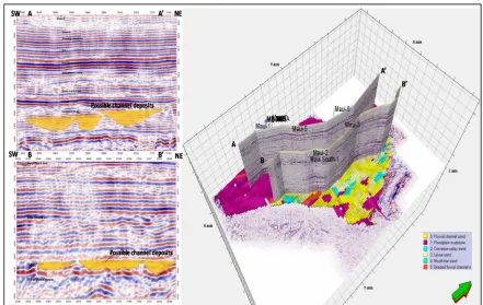
282
283
3.4.1. Sequence I
284
Sequence I was recognized in all studied wells and its minimum thickness ranges from 30-60 m.
285
The lower boundary could not be precisely delineated as it interfingers with the underlying North
286
Cape Formation. Its upper boundary consisted of a regional-scale erosional surface. Major facies
287
associations of the Sequence I was Ephemeral Fluvial Channels mainly meandering deposits.
288
Sequence I was interpreted to be a Type-I Falling Stage Systems Tract FSST) boundary marked by an
289
unconformity. This was characterized by stream rejuvenation and fluvial incision, sedimentary
290
bypass of the shelf, and abrupt basin-ward shift of facies and coastal onlap. This might be formed
291
when the rate of eustatic fall exceeds the rate of basin subsidence at the depositional shoreline break,
292
producing a relative fall in sea level below the position of the paleoshoreline [61].
293
294
3.4.1.1. Depositional architecture
295
Sequence I displayed a progradational facies succession. The base was dominated by
296
fine-grained shallow marine deposits of the North Cape Formation that were overlain by fluvial
297
strata. While fluvial flow was dominantly from NE to SW, indicating sediment transport towards the
298
southern border of the basin.
299
Fluvial deposits were laterally and vertically adjacent, producing a complex depositional
300
architecture. Both single storied and stacked meandering sand packages occur within the sequence
301
consisting of 2-15m thick and >1 km in horizontal directions towards the X and Y axis of the model,
302
the upper boundaries were fluvial scour surfaces with <5 m of erosional relief into the Aeolian
303
deposits. Wherever single stack fluvial erosion was substantial, multiple channel deposits were
304
severely to completely truncated (Fig.11).
305
306
Figure.12. 3D geocellular facies distribution of the Farewell Formation. The image below represents the facies
307
model in SIMBOX view, vividly displaying interpreted facies in X-Y-Z axis within the facies model of the
308
Farewell Formation.
309
3.4.2. Sequence II
313
Sequence II ranged from 30-40 m in thickness. The lower boundary of Sequence II comprised a
314
regional scale unconformity that was identified in the well logs and interpreted to be a Lowstand
315
Systems Tract (LST) within the depositional cycles of the Farewell Formation. Its upper boundary
316
was also defined by an erosional surface that can be correlated throughout the basin (Fig.11). Two
317
facies associations were distinguished within this sequence, representing (1) Braided Fluvial
318
Channel Belts and (2) Overbank Environments.
319
320
3.4.2.1. Depositional Architecture
321
Sequence II was uniform in terms of fluvial facies architecture throughout the entire basin,
322
precluding the recognition of distinct internal stratigraphic intervals. This sequence represented a
323
northwestward-flowing braided fluvial system developed on a widespread alluvial plain. Its
324
geological record was characterized by a succession of sandstone bodies (braided channel belt
325
deposits) partially separated by thin and discontinuous fine-grained, floodplain deposits. Therefore,
326
Sequence II consisted of vertical and lateral juxtaposition of several sandstone bodies produced by
327
successive avulsion episodes, similar to the fluvial accumulation models described elsewhere for
328
braided fluvial systems [41, 68]. The minor quantity of flood plain deposits indicated that overbank
329
sedimentation was either restricted or the resultant deposits were reworked by fluvial channels. The
330
scarcity of mudstone intraclasts at the base of the sandstone bodies supported the former hypothesis,
331
i.e. floodplains were poorly developed. Therefore sequence-II was interpreted to be regressive, being
332
a Lowstand Systems Tract (LST).
333
334
Figure.13. Vertical Proportion Curve (VPC) for all possible geobodies within the Farewell Formation. (a) VPC of
335
fluvial (meandering) channel sands, (b) VPC of floodplain mudstone, (c) VPC of crevasse splay sands, (d) VPC
336
of levee sand, (e) VPC of mouth bar sands, (f) VPC of braided channel sands.
337
338
3.5. 3D-Modeling Approach
339
The Facies Composite algorithm in Petrel was adopted to construct facies model of the Farewell
340
Formation, which is an object-based facies modeling technique that can be used for a wide range of
341
heterogeneities and depositional environments. The basic concept of the Facies Composite algorithm
342
was that the facies within a grid model can be subdivided into a background facies and one or more
343
object facies, which can have different shapes, sizes and orientations [22, 69-70]. The Facies
344
Composite algorithm models the geometries and distribution of the object facies [23, 69, 71]. Facies
345
sizes and shapes were drawn from a user-specified distribution that might differ locally within the
346
reservoir [23, 72-74]. The entire process was based on a 3D geocellular modeling grid for the study
347
Following the structural restoration, the digital reconstruction of the boundaries of the
349
sedimentary bodies involved the following steps: (a) visual construction of structured geobodies
350
along with defined geometries of the interpreted lithology (b) variogram analysis of the geobody
351
dimensions (c) incorporation of the paleo-depositional interpretation within each geobody and (d)
352
construction of a consistent 3D subsurface-based model. The process of reconstructing the
353
sedimentary bodies was used as a quality control on the existing field correlation. This
354
reconstruction supported the interpreted rectilinear geometry of the channeled sandbodies.
355
356
Figure.14. Facies proportions thickness Vs probability of occurrence for the Farewell Formation. Colors
357
represent different geobodies interpreted in the model.
358
359
3.6. Modeling Grids and Constraints
360
For the 3D lithology models, seismic-derived structure maps were used to define the base and
361
the top of the stratigraphic interval of the formation. The top of the model was then assigned within
362
the layering algorithm denoting arbitrary layer number 110, and the base of the model being 120,
363
which was around 100m in thickness on an average along the studied wells (Fig.12). Between the
364
reservoir, 9 zones of equal thickness were constructed for better enhancement (along the vertical
365
accurately model the lithologic variability within the reservoir. For the construction of the modeled
367
grid, following process was used to create the vertical proportion curve.
368
A vertical proportion curve (VPC) (Fig.13) is a cumulative probability plot that shows the
369
percentage of lithology versus depth. In this study we characterized VPC analysis considering all the
370
studied wells within the gridded model. To create the vertical proportion curve, the interval
371
between Farewell Formation was subdivided into an equal number of approximately 10m thick
372
layers.
373
For this reason, proportional layers were defined within this stratigraphic interval in the well
374
logs. The proportional layers had an approximate thickness of 10m in general but the thickness
375
varied laterally, from well to well, given the same number of layers per reservoir zone on each well
376
log. For each layer, the percentage of each lithology (sandstone, shale, coal) in that interval was
377
determined from the well logs. The original well-log data were used in this analysis. By combining
378
the well log data for each layer in this way, a vertical proportion curve was created that provides a
379
1D vertical trend to show how the lithology percentages vary with respect to depth in this study
380
area.
381
From the VPC, it was evident that 6 different geobodies were three-dimensionally distributed
382
along the Farewell Formation. From figure 13(a) meandering channel sand proportion curve was
383
interpreted. We interpreted that, probability of occurrence for meandering channel sands were
384
varying in different layers of the model. Layer 111-115 had higher probability of occurrence whereas
385
layers from 116-118 have 20-29% probability of occurrence within the model. Layer 119-120 had only
386
10-15% probability of having meandering channel sand deposits. For floodplain mudstones, highest
387
percentage of occurrence concentrated within the deeper layers (30-60%) (Fig.13b). For crevasse
388
splay sands, probability of occurrence was very low; around 10% for all the interpreted layers of the
389
Farewell Formation (Fig.13c). Figure 13d represented VPC for levee sands. Probability of occurrence
390
for levee sands within the model was very low in the deeper layers (2-8%) compared to that of the
391
shallower layers (5-9%). Mouth bar sands had a distribution of lower VPC all along the modeled
392
layers (Fig.13e). Braided channel sands had higher probability of occurrence in the shallow layers,
393
compared to the meadering ones.
394
To create the 3D model grid based on the VPC, facies thickness maps were generated for each of
395
the reservoir zones. The isopach maps were added to a single reference surface in the model to create
396
the additional structure maps (reservoir model surfaces) needed to define the 3D model grid or
397
framework. This process ensured all structure maps to be consistent with the structural trends.
398
A detailed 3D facies model of 300,000 geo-gridded cells was created for 3D facies modeling.
399
Fine-scale layers were distributed proportionally between the key stratigraphic surfaces. Each fine
400
layer was approximately 10m thick to capture the stratigraphic detail of both meandering and
401
braided deposits. Lateral cell dimensions of 50m X 50m were used to capture the details of the lateral
402
distribution of the fluvial deposits and in order to have several cells between wells.
403
To honour the lithologic variability in wells, lithology logs were created for each well and
404
subsequently upscaled to the resolution of the model grid and used in the modeling process. To
405
create the lithology logs for all 4 wells, various cutoffs for the well-log data were used for each
406
lithology for generating point attributes for each well, that later were incorporated into the 3D
407
model. It was to be noted that in the study area, values less than 70 API units on the gamma-ray log
408
was defined as sandstones (North and Boering 1999; Rider 1990). Values greater than 70-90 API units
409
on the gamma-ray log was defined as silty sandstone to clayey siltstone and values above that were
410
all termed as shales.
411
During the modeling process, the scaled sand-shale ratio volume was used as a conditioning
412
parameter to control the spatial distribution of sandstone bodies or sandstone lithology within the
413
3D models. The calculations were performed using the Data Analysis plug-in of Petrel (Fig.14). As a
414
result, if a modeled layer within the Farewell reservoir exhibits a high percentage of sandstone, the
415
corresponding reservoir layer in the 3D model will have a high percentage of sandstone.
416
For the object-based lithology (sandstone, shale) modeling, the dimensions of sand bodies were
417
75-78]. For the indicator based modeling, the spatial correlation of the lithologies of the Farewell
419
Formation was quantitatively analyzed through variogram analysis. Experimental variograms were
420
calculated separately for each reservoir zone and lithology and were fitted with exponential and
421
spherical variogram models. Correlation lengths of the model variograms ranged from
422
approximately 25-35000 m parallel to paleoflow (Northeast to Southwest) in the major direction and
423
424
Figure.15. Object geometries (a-f) of the interpreted geobodies of the Farewell Formation. Each geobody
425
represents its spatial distribution within the formation along the X-Y-Z axis of the modeled grid. Braided
426
channel sands to meandering channel deposits have been modeled for the analysis. Figure 15g represent the
427
entire facies model combined with all possible geobodies of the Farewell Formation, Maui Gas Field.
428
429
around 12-15000 m perpendicular to paleoflow in the minor direction and vertically around 100 m
430
on an average within the studied wells (Fig.15). The few zones with longer vertical correlation
431
rather than individual mouth bars. It was important to note that the correlation lengths do not
433
directly provide information on the dimensions, geometry and sinuosity of the fluvial deposits.
434
We used sequential-indicator simulation and conditioned it to fit with the object based geobody
435
modeling [30, 75] to generate a 3D facies model for the Farewell Formation. A value for lithology
436
was simulated in each cell of the model based on probabilities calculated from well data and
437
user-defined inputs. The percentages of each lithology were defined for each zone based on well
438
data.
439
For the sequential-indicator simulation model (indicator-based model), the global volume
440
fraction for sandstone was 45% sandstone and 55% shale. Because indicator-based simulation used
441
variograms (a two-point statistics) to incorporate the spatial correlation of the reservoir lithologies,
442
the geometries of channel sand bars were, as expected, not reproduced using this method. However,
443
the general distribution of sandstone honored all the constraints. The lower portion of the facies
444
model (layer 115-120) of the indicator-based model was composed primarily of discontinuous
445
sandstones and shales which whereas stacked and more continuous sandstone and interbedded
446
shale intervals were more common in the upper part of the facies model. The upper part was
447
therefore denominated as possible braided stacked channel sands and the lower being multistoried
448
meandering channel sand deposits. Relatively small and discontinuous sand bodies were observed
449
throughout the modeled interval.
450
451
3.7. Object geometry
452
The geometrical properties for each selected facies association in all zones were set by defining
453
different and reasonable geometries (Fig.15a-f). Distributary channel, the main H/C bearing facies,
454
was defined as a backbone which was a variant of the axial shape where the object was deformed
455
locally to follow a direction parameter. Its thickness and width remained constant along axis and the
456
cross sectional formed as U shapes (Fig.15f). The overbank was also defined as an axial shape with
457
constant thickness and slight width variation. The mouth bar (Fig.15b) was defined as an axial lobe
458
body whose width increased then decreased along axis with a lentoid cross sectional form. It was
459
worth noting that these definitions do not determine the size or orientation of the bodies, they only
460
specify a prototype shape for the object and this shape was then rescaled and orientated using the
461
size and orientation attribute values.
462
Evidence of possible multi-storey stacking within the sand-body profile was usually in the form
463
of a minor gamma peaks that might result from thin units of fine-grained sediment or, more likely,
464
horizons of intra-formational mud clasts resting on erosion surfaces at the bases of stacked storeys.
465
Such sandbodies range in thickness from around 10 m up to over 20 m (Fig.15a/f). In the object-based
466
facies modeling, it was necessary to define facies body log to split a multi-storey channel interval
467
into different facies objects and get a better statistics of properties and thus a better simulation result
468
[79-80]. The body division results were showed along with the prospective major and minor
469
directions in figure 15 (a-f).
470
471
3.8. Object-based simulation of the geobodies
472
Object-based simulation involves defining lithology (or facies, architectural element) objects
473
with a range of dimensions and characteristic shapes that were used to populate the 3D model
474
[80-81]. This method honored geologic rules for stacking patterns and erosion and user-defined
475
shapes that, in some cases, can produce more geologically realistic models than other modeling
476
methods [30, 75].
477
For this study, the modeled elements were crescent-shaped objects that represent the main
478
reservoir elements (mouth bars) within the studied formation. The thickness of individual channel
479
sands within the grid was modeled using a triangular distribution with values ranging from 2-15m
480
with an average of 8.5m. Individual bar widths range from 200-400m with an average of 300m. The
481
mouth-bar shape was modeled as a scalable crescent-shaped body based on the study of
482
paleo-channel reconstructions of mouth bars [23, 77-78]. Therefore this method used objects with
483
not used) which resulted in improved model predictions as compared to the corresponding
485
indicator-based models.
486
487
Figure.16. Seismic attribute (coherence) showing the paleochannels within the Farewell Formation. Solid black
488
lines are possible fluvial channels as interpreted on the Z slice of the seismic cube.
489
490
To simplify the modeling process, separate stochastic object-based models were generated for
491
each lithology and then merged to create the final lithology model. The two sandstone and shale
492
models were constructed using the same ranges of object dimensions for the sandstone bodies but
493
used different object orientations. These models were then merged to create a final model with point
494
orientations that were consistent with outcrop measurements. The orientations of the geobodies
495
were consistent with the approximate paleoflow direction of the Farewell Formation of the Maui Gas
496
Field. The range in orientations produced crescent-shaped and lenticular objects that represent bar
497
deposits on opposite sides of a sinuous meandering stream system. Using this approach,
498
crescent-shaped sand bar objects were modeled, along with the fluvial channels; therefore, the
499
sinuosity, amplitude and wavelength of the inferred channels that deposited the sandstones were
500
not used as input into the modeling process. The sinuosity of Farewell Formation fluvial channels
501
was estimated to be approximately 1.7–1.9 based on sandstone body width-to-thickness ratios and
502
amplitude and wavelength were not modeled explicitly, the modeled object dimensions and
504
orientations were consistent with the previous studies [23, 31, 77, 82]. With the combination of
505
indicator and object based modeling, the final outputs were constrained by well data and seismic
506
picks and resulted in a 3D geobody grid for the studied formation.
507
508
Figure.17. Vertical seismic profiles (in TWT) for the Farewell Formation. AA' and BB' profiles represent major
509
channel forms along the facies model of the formation. Note that the interpreted paleochannels (BB') have more
510
width-thickness ratio compared that of the westward profile (AA').
511
512
3.9. 3D Facies Architecture based on Seismo-sedimentological Interpretation
513
A number of investigations were published on facies architecture analysis based on outcrop,
514
well, seismic, and experimental data [45, 52, 83-87]. In this study, we applied seismic sedimentology
515
to extend the well data study to the entire block covered by 3-D seismic survey and to provide more
516
detailed sedimentary facies architecture mapping [29, 88-90]. Stratal slicing and 90°-phasing were
517
two key techniques used in seismic sedimentology analysis [29, 89].
518
Using horizontal seismic patterns within a small travel-time window that followed the
519
sedimentary facies, a stratal slice could reveal more detailed geobody distributions and sedimentary
520
facies in much higher resolution with less ambiguity than that was possible by using classic seismic
521
stratigraphy [89-90].
522
523
3.9.1. Spatial distribution and temporal evolution of incised valleys
524
The incised valley fill was used to identify the sediment transport direction, deduce the
525
sedimentary dispersal system, and served as a potential high-quality reservoir [91-94]. As a typical
526
sand-prone fill and the main drainage system in the study area, the spatial distribution and temporal
527
evolution of incised valleys were investigated in great detail.
528
529
3.9.1.1. Spatial distribution of incised valleys
530
Figure 16 explained the spatial distribution of incised valleys using coherence attribute.
531
Coherence attribute was used in the study because of its effectiveness in identifying edge detection
532
along with possible channel boundaries. In figure 16a to figure 16b, the bottom of each figure was
533
and crossline cross sections, respectively, which were used for interpreting the spatial distribution of
535
incised valleys.
536
Moving the Z slices on the seismic sections from figure 16a to 16b, the numbers of incised
537
valleys changes and their width-to-thickness ratio was evident from upstream to downstream region
538
of the stratal slice(Fig.16). In figure 16a, at least 9 prominent incised valley fills were interpreted on
539
the seismic section with multiple, very strong converging and branching belt-shaped amplitude
540
anomalies in the slice from upstream to downstream (NE-SW). The anomalies had a close
541
corresponding relationship with incised valleys on the seismic section, indicating the planar
542
distribution of multiple incised valleys.
543
11 incised valleys were interpreted in figure 16b. There were also combined channel forms,
544
branching out from main channel seen in the seismic slice. This corresponds to high amplitude
545
anomalies (coherence attribute) in the stratal slice. It was also evident that the width-to-thickness
546
ratio of incised valleys gradually decreases from upstream to downstream.
547
548
3.9.1.2 Temporal evolution of incised valley fills
549
Representative seismic profiles shown in 3-D visualization from the Farewell Formation
550
sequences revealed the temporal evolution of the incised valley fills from the bottom to top
551
boundary (Fig.17). In figure 17, the bottom of the illustration was the vertical slice showing the
552
reflection amplitude of different stages of the two major sequences. The higher amplitudes were
553
characterized by channel sands distributed spatially.
554
The belt-shaped high amplitudes reflected the difference of incised valley fills in the stratal
555
slices, indicating the differences in width, sinuosity, continuity, and extended length (Fig.17),
556
reflecting the hydrodynamic change and temporal evolution of an incised valley fill. The incised
557
valleys tend to be of broad and straight amplitude anomalies. In comparison, it was observed that
558
incised valleys were characterized by narrow and meandering channels; the number of incised
559
valleys obviously increases while their width decreases. The incised valleys actively developed in
560
figure 17 were almost faded in the bottom vertical slice; whereas incised valleys developed at the top
561
slice were characterized by branching and converging. From the interpretation of channel
562
distribution and occurrence, the variations in number, width, and sinuosity of incised valleys
563
indicated the evolution of incised valleys from initiation to extinction [91, 94-95].
564
5. Conclusions
565
The following conclusions can be made from this study:-
566
1) We identified three major depositional facies distributed over the paleo-environmental setup
567
of the Farewell Formation. It was also observed that the current workflow of facies occurrence and
568
probability according to the geological knowledge-base and grid sequencing showed considerable
569
improvements within the modeled region of the Maui Gas Field.
570
(2) The Farewell reservoir was interpreted to be of fluvial paleo-environment in origin.
571
Interpretations lead us to believe that about 45% of the depositional facies are of channel sandstone
572
origin and the rest 55% are floodplain/overbank shales.
573
(3) The Farewell model was sequence stratigraphically interpreted to be of Type-I origin having
574
Lowstand Systems Tract (LST) of fluvial origin.
575
(4) It was also observed that the lower portion of the geobody facies model (layer 115-120) was
576
composed primarily of discontinuous sandstones and shales. Sandstone and interbedded shale
577
intervals were more common in the upper part of the facies model. The upper part was therefore
578
denominated as possible braided stacked channel sands and the lower being multistoried
579
meandering channel sand deposits.
580
(5) We modeled at least eleven prominent incised valley fills on the seismic section with
581
multiple, very strong converging and branching belt-shaped amplitude anomalies in the slice from
582
upstream to downstream (NE-SW). The anomalies had close corresponding relationship with
583
There were combined channel-forms, branching out from main channel corresponding to high
585
amplitude anomalies predicted to be higher quality reservoir sands.
586
(6) The geobody modeling process had effective advantage of quantitative propagation of
587
uncertainty via the object-based algorithm of the identified geobodies distributed across of the
588
formation. Thus the facies model was interpreted to be used as a significant new tool for future
589
studies on deeper reservoirs and their development strategies for better production.
590
Acknowledgments: This study is funded as part of the doctoral research (GRS-2015) at the Department of
591
Geological Sciences, Universiti Brunei Darussalam (UBD). The authors would like to thank Ministry of
592
Business, Innovation and Employment (MBIE), New Zealand for providing dataset containing 3D seismic, well
593
logs and associated reports required for this study. Schlumberger is greatly acknowledged for supporting us
594
with Petrel G&G software v.2013.1.
595
Author Contributions: AKM Eahsanul Haque (A. E. H.) developed the 3D geobody modeling concept for the
596
reservoir, workflow and static modeling parameters; Md Aminul Islam (M. A. I.) improved the well log facies
597
analysis and Mohamed Ragab Shalaby (M. R. S.) contributed to correct the manuscript.
598
Conflicts of Interest: The authors declare no conflict of interest.
599
References
600
1. 1. Childs, C.; Nicol A.; Walsh J. J. The growth and propagation of synsdimentary faults. Journal of
601
Structural Geology2003, 25(4), 633–648, doi.org/10.1016/S0191-8141(02)00054-8.
602
2. Reilly, C.; Nicol A.; Walsh J. J. Evolution of faulting and plate boundary deformation in the Southern
603
Taranaki Basin, New Zealand. Tectonophysics2015, 651, 1–18, doi.org/10.1016/j.tecto.2015.02.009.
604
3. Uruski, C. I. Deepwater Taranaki, New Zealand: structural development and petroleum potential.
605
Exploration Geophysics2008, 39(2), 94-107, doi.org/10.1071/EG08013.
606
4. Mcbeath, D. M. Gas-condensate fields of the Taranaki basin, New Zealand. New Zealand Journal of Geology
607
and Geophysics1977, 20(1), 99–127.
608
5. Kamp, P. J. J.; Vonk, A, J., Bland, K. J.; Hansen, R. J.; Hendy, A. J. W.; Mcintyre, A. P.; Ngatai, M.;
609
Cartwright, S. J.; Hayton, S.; Nelson, C. S. Neogene stratigraphic architecture and tectonic evolution of
610
Wanganui, King Country, and eastern Taranaki Basins, New Zealand. New Zealand Journal of Geology and
611
Geophysics2004, 47(4): 625-644, doi.org/10.1080/00288306.2004.9515080.
612
6. King, P. R.; Thrasher, G. P. Cretaceous–Cenozoic geology and petroleum systems of the Taranaki Basin,
613
New Zealand. Institute of Geological and Nuclear Sciences, Lower Hutt, New Zealand, 1996, 13(2).
614
7. King, P. R. Polyphase evolution of the Taranaki Basin, New Zealand: changes in sedimentary and
615
Structural style. New Zealand Oil Exploration Conference Proceedings, Wellington, 1990, 134–150.
616
8. King, P. R.; Browne, G. H.; Slatt, R. M.; Diridoni, J. L. High resolution sequence stratigraphy of Miocene
617
Deepwater clastic outcrops, Taranaki coast, New Zealand. American Association of Petroleum Geologists
618
International Conference and Exhibition, 1995, 79, CONF-950995.
619
9. Skalle, P.; Aamodt, A. Knowledge-based decision support in oil well drilling. International Conference on
620
Intelligent Information Processing, 2004, 443-455.
621
10. Luthi, S. (2001). Geological well logs: Their use in reservoir modeling. Springer Science & Business Media,
622
2001.
623
11. Higgs, K. E.; Funnell, R. H.; Reyes, A. G. Changes in reservoir heterogeneity and quality as a response to
624
high partial pressures of CO 2 in a gas reservoir, New Zealand. Marine and Petroleum Geology 2013, 48,
625
293-322, doi.org/10.1016/j.marpetgeo.2013.08.005.
626
12. Higgs, K. E.; Zwingmann, H.; Reyes, A. G.; Funnell, R. H. Diagenesis, porosity evolution, and petroleum
627
emplacement in tight gas reservoirs, Taranaki Basin, New Zealand. Journal of Sedimentary Research
628
2007, 77(12), 1003-1025, doi.org/10.2110/jsr.2007.095.
629
13. Martin, K. R.; Baker, J. C.; Hamilton, P. J.; Thrasher, G. P. Diagenesis and reservoir quality of paleocene
630
sandstones in the Kupe South field, Taranaki Basin, New Zealand. AAPG bulletin1994, 78(4), 624-643.
631
14. Strogen D. P.; Bland K. J.; Baur J. R. Rift to drift on the edge of Gondwana: Cretaceous-Eocene
632
paleogeographic evolution of the Taranaki Basin, New Zealand. Geosciences New Zealand Annual
633
conference, Wellington, New Zealand, 2014, 1–17.
634
15. Laird, M. G. Cretaceous continental rifts: New Zealand region. Sedimentary basins of the world 1993, 2,
635
16. Stagpoole, V. M.; Nicol A. Regional structure and kine-matic history of a large subduction back thrust:
637
Taranaki Fault, New Zealand. Journal of Geology and Geophysics 2008, 113(B1), 769–775,
638
doi.org/10.1029/2007JB005170.
639
17. Holt, W. E.; Stern T. A. Subduction, platform subsidence, and foreland thrust loading: The late Tertiary
640
development of Taranaki Basin, New Zealand. Tectonics 1994, 13(5), 1068–1092,
641
doi.org/10.1029/94TC00454.
642
18. King, P. R.; Thrasher G. P. Post-Eocene development of the Taranaki Basin, New Zealand: Convergent
643
overprint of a passive margin. Geology and geophysics of continental margins 1992, 53, 93–118.
644
19. Bussell, M. R. Seismic interpretation of the Moki Formation on the Maui 3D survey, Taranaki Basin. New
645
Zealand Petroleum Conference proceedings, Sydney, Australia, 1994, 240-255.
646
20. King, P. R.; Robinson, P. R. An overview of Taranaki region geology, New Zealand. Energy Exploration &
647
Exploitation1988, 6(3), 213–232.
648
21. Haque, A. E.; Islam, M. A.; Shalaby, M. R. Structural Modeling of the Maui Gas Field, Taranaki Basin, New
649
Zealand. Journal of Petroleum Exploration and Development 2016, 43(6), 965-975,
650
doi.org/10.1016/S1876-3804(16)30114-8.
651
22. Pyrcz, M. J.; Mchargue, T.; Clark J.; Sullivan, M.; Strebelle, S. Event-based geostatistical Modeling:
652
description and applications. Geostatistics 2012, 27-38, doi.org/10.1007/978-94-007-4153-9_3.
653
23. Pyrcz, M. J.; Sech R. P.; Covault, J. A.; Willis, B. J.; Sylvester, Z.; Sun, T. Stratigraphic rule-based reservoir
654
modeling. Bulletin of Canadian Petroleum Geology2015, 63(4): 287-303.
655
24. Keeton, G. I.; Pranter, M. J.; Cole, R. D.; Edmund, R. Stratigraphic architecture of fluvial deposits from
656
borehole images, spectral-gamma-ray response, and outcrop analogs, Piceance Basin, Colorado. AAPG
657
Bulletin2015, 99(10), 1929-1956.
658
25. Deutsch, C. V. Geostatistical Reservoir Modelling, Oxford University Press, 2002, pp. 376.
659
26. Strebelle, S.; Zhang T. Non-stationary multiple-point geostatistical models. Geostatistics Banff 20042005
660
235-244.
661
27. Goovaerts, P. (2006). Geostatistical modeling of the spaces of local, spatial, and response uncertainty for
662
continuous petrophysical properties. In Stochastic modeling and geostatistics: Principles, methods, and case
663
studies, volume II: AAPG Computer Applications in Geology; T. C. Coburn, T. C.; Yarus, J. M.; Chambers, R. L,
664
AAPG, USA, 2007; 2(5), pp. 59–79, doi.org/10.1306/1063807CA53229.
665
28. Mikes, D.; Barzandji, O. H. M.; Bruining, J.; Geel, C.R. Upscaling of small-scale heterogeneities to flow
666
units for reservoir modeling. Mar. Pet. Geol.2006, 23(9), 931-942, doi.org/10.1016/j.marpetgeo.2005.06.005.
667
29. Zhang, T.; Zhang, X.; Lin, C.; Yu, J.; Zhang, S. Seismic sedimentology interpretation method of
668
meandering fluvial reservoir: From model to real data. Journal of Earth Science 2015, 26(4):598-606,
669
doi.org/10.1007/s12583-015-0572-5.
670
30. Deutsch, C. V.; Journel A. G. Geostatistical Software Library and user’s guide, Oxford University Press,
671
New York, pp. 369.
672
31. Pranter, M. J.; Ellison A. I.; Cole R. D.; Patterson P. E. Analysis and modelling of intermediate-scale
673
reservoir heterogeneity based on a fluvial point-bar outcrop analogue, Williams Fork Formation, Piceance
674
Basin, Colorado. AAPG Bulletin2007, 91(7), 1025–51, doi.org/ 10.1306/02010706102.
675
32. Bal, A. A. Estuarine to fluvial transition: the Cretaceous/Tertiary "Puponga" Coal Measures in the
676
Pakawau Group, northwest Nelson. B.Sc (Hons) thesis, University of Canterbury, New Zealand, 1992.
677
33. Bal, A. A. (1994). Cessation of Tasman Sea spreading recorded as a sequence stratigraphy: interpretation of
678
an early Paleocene unconformity in the Pakawau subbasin, NW Nelson, New Zealand. In The evolution of
679
the Tasman Sea Basin, Proceedings of the Tasman Sea Conference, Christchurch, New Zealand, 1994, Van
680
der Lingen, G. J.; Swanson, K. M.; Muir, R. J. Balkema Publishers, pp. 23-30.
681
34. Bal, A. A. Disparate hydrocarbon generation potential and maturation profiles of Pakawau Group source
682
coals: implications for Taranaki Basin exploration, New Zealand. In Petroleum Exploration Conference
683
Proceedings, Ministry of Economic Development, Wellington, New Zealand, 1994, pp. 322–337.
684
35. Thrasher, G. P. Late Cretaceous source rocks of Taranaki Basin. New Zealand Oil Exploration Conference
685
proceedings, Crown Operations Group, Energy and Resources Division, 1991, pp. 147-154.
686
36. Benvenuti, M.; Del C., S. Facies and sequence stratigraphic modeling of a Upper Pliocene–Lower
687
Pleistocene fluvial succession (Valdelsa Basin, central Italy). Sedimentary Geology 2013, 294, 303–314,
688
37. Fanti, F.; Catuneanu, O. Fluvial sequence stratigraphy: the wapiti Formation,West- Central Alberta,
690
Canada. Journal of Sedimentary Research 2010, 80(4), 320–338.
691
38. Chakraborty, T. Reconstruction of fluvial bars from the Proterozoic Mancheral Quartzite,
692
Pranhita–Godavari, India. In Fluvial Sedimentology VI, Int. Assoc. Sediment. Special Publication, 1999, 28,
693
pp. 451–466.
694
39. Miall, A. D. Facies architecture in clastic sedimentary basins. New perspectives in basin analysis 1988, 67-81.
695
40. Miall, A. D. Reservoir heterogeneities in fluvial sandstones: lessons from outcrop studies. AAPG Bulletin
696
1988, 72(6), 682-97.
697
41. Miall, A. D. The Geology of Fluvial Deposits: Sedimentary Facies, Basin Analysis and Petroleum Geology.
698
Springer-Verlag, New York, USA, 2013, pp. 495-519.
699
42. North, C. P., Taylor, K. S. Ephemeral–fluvial deposits: integrated outcrop and simulation studies reveal
700
complexity. AAPG Bulletin 1996, 80(6), 811–830,
701
43. Aitken, J. F.; Flint, S. The application of sequence stratigraphy to fluvial systems: an example from the Late
702
Carboniferous of the Appalachians. Sedimentology1995, 42, 3–30.
703
44. Bristow, C.S. Brahmaputra river: channel migration and deposition. In Recent Developments in Fluvial
704
Sedimentology, Ethridge, F.G.; Flores, R. M.; Harvey, M. D, SEPM Special Publication, 1987, 39, pp. 83–91.
705
45. Scherer, C. M.; Lavina E. L.; Dias F. D. C.; Oliveira F. M.; Bongiolo D. E.; Aguiar E. S. Stratigraphy and
706
facies architecture of the fluvial–aeolian–lacustrine Sergi Formation (Upper Jurassic), Recôncavo Basin,
707
Brazil. Sedimentary Geology 2007, 194(3), 169-193, doi.org/10.1016/j.sedgeo.2006.06.002.
708
46. Gulliford, A.R.; Flint, S.S.; Hodgson, D.M. Testing applicability of models of distributive fluvial systems or
709
trunk rivers in ephemeral systems: reconstructing 3-D fluvial architecture in the Beaufort Group, South
710
Africa. Journal of Sedimentary Research 2014, 84(12), 1147-1169, doi.org/10.2110/jsr.2014.88.
711
47. Ékes, C. Bedload-transported pedogenic mud aggregates in the Lower Old Red Sandstone in southwest
712
Wales. Journal of the Geological Society1989, 150(3), 469-71.
713
48. Rust, B. R,; Nanson G. C. Bedload transport of mud as pedogenic aggregates in modern and ancient rivers.
714
Sedimentology1989, 36(2), 291-306.
715
49. Fielding, C. R.; Allen J. P.; Alexander J.; Gibling M. R. Facies model for fluvial systems in the seasonal
716
tropics and subtropics. Geology20009, 37(7), 623-6.
717
50. Bridge, J. S. Description and interpretation of fluvial deposits: a critical perspective. Sedimentology1993,
718
40(4), 801-810.
719
51. Sahoo, H.; Gani, M. R.; Hampson, G. J.; Gani, N. D.; Ranson, A. Facies-to sandbody-scale heterogeneity in
720
a tight-gas fluvial reservoir analog: Blackhawk Formation, Wasatch Plateau, Utah, USA. Marine and
721
Petroleum Geology 2016, 78, 48-69, doi.org/10.1016/j.marpetgeo.2016.02.005.
722
52. Blum, M. Scaling relationships between fluvial channel fills, channel-belt sand bodies and drainage basins,
723
with implications for the Mannville Group, Alberta Foreland Basin. AAPG Annual Convention and
724
Exhibition, 2015.
725
53. Pisel, J. R.; Pyles D. R. On The Relationship Between Fluvial Channel-Belt Morphology And Internal
726
Heterogeneity: Insights From Satellite, Seismic, Numerical, And Outcrop Datasets. Doctor of Philosophy
727
Thesis, Colorado School of Mines, USA, 2015..
728
54. Willis, B. J.; Sech R.; Sun T.; Pyrcz M. Predicting Facies Patterns within Fluvial Channel Belts. Inagu Fall
729
Meeting Abstracts, 2014, 1, 3529.
730
55. Godin, P. D. Fining-upward cycles in the sandy braided-river deposits of the Westwater Canyon Member
731
(Upper Jurassic), Morrison Formation, New Mexico. Sedimentary Geology1991, 70(1), 61-82.
732
56. Colombera, L.; Mountney N. P.; Felletti F.; mccaffrey W. D. Models for guiding and ranking well-to-well
733
correlations of channel bodies in fluvial reservoirs. AAPG Bulletin 2014, 98(10), 1943-1965,
734
doi.org/10.1306/05061413153.
735
57. Lowe, D. G.; Arnott R. W. Composition and Architecture of Braided and Sheetflood-Dominated
736
Ephemeral Fluvial Strata In the Cambrian–Ordovician Potsdam Group: A Case Example of the
737
Morphodynamics of Early Phanerozoic Fluvial Systems and Climate Change. Journal of Sedimentary
738
Research 2016, 86(6), 587-612, doi.org/10.2110/jsr.2016.39.
739
58. Van Wagoner, J. C.; Mitchum R. M.; Campion K. M.; Rahmanian V. D. Siliciclastic sequence stratigraphy in
740
well logs, cores, and outcrops: concepts for high-resolution correlation of time and facies, AAPG Methods