Technical Methodology for ASTER Global Water Body Data Base

1

Technical Methodology for ASTER Global Water Body Data Base

1 _{Sensor Information Laboratory Corp. ,2-23-36 Shihaugaoka, Tsukubamirai, Ibaraki Japan}

2 _{Institute of Advanced Industrial Science and Technology(AIST), 1-1-1, Umezono, Tsukuba, Ibaraki, Japan,} 3 _{Research Center for Advanced Science and Technology,University of Tokyo, Tokyo, Japan}

* Correspondence: [email protected]; Tel: +81-297-21-7244

Abstract: A waterbody detection technique is an essential part of digital elevation model (DEM) generation to delineate land-water boundaries and set flattened elevations. This paper describes the technical methodology for improving the initial based waterbody data that are created during production of the ASTER GDEM, because without improvement such tile-based waterbody data are not suitable for incorporating into the new ASTER GDEM Version 3. Waterbodies are classified into three categories: sea, lake, and river. For sea-waterbodies, the effect of sea ice is removed to better delineate sea shorelines in high latitude areas, because sea ice prevents accurate delineation of sea shorelines. For lake-waterbodies, the major part of the processing is to set the unique elevation value for each lake using a mosaic image that covers the entire lake area. Rivers present a unique challenge, because their elevations gradually step down from upstream to downstream. Initially, visual inspection is required to separate rivers from lakes. A stepwise elevation assignment, with a step of one meter, is carried out by manual or automated methods, depending on the situation. The ASTER GWBD product consists of a global set of 1º latitude-by-1º longitude tiles containing water body attribute and elevation data files in geographic latitude and longitude coordinates and with one arc second posting. Each tile contains 3601-by-3601 data points. All improved waterbody elevation data are incorporated into the ASTER GDEM to reflect the improved results.

Keywords: ASTER instrument, stereo, digital elevation model, global database, optical sensor, water body detection.

I. Introduction

The Advanced Spaceborne Thermal Emission and Reflection radiometer (ASTER) is an advanced multispectral imaging sensor that was launched on board the Terra spacecraft in December, 1999 [1,2]. ASTER has an along-track stereoscopic viewing capability in its visible and near-infrared (VNIR) bands at 15-m spatial resolution with a base-to-height ratio of 0.6. Because of ASTER’s excellent satellite ephemeris and instrument parameters [3ー6], this along-track stereoscopic viewing capability makes it possible to generate excellent digital elevation model (DEM) data products from ASTER data without referring to ground control points (GCPs) for individual scenes.

After nearly a decade of ASTER data acquisition, sufficient cloud-free data had been acquired such that it was possible to create a global DEM from ASTER data (ASTER GDEM). Versions 1 and 2 of the ASTER GDEM, based on 1.2 and 1.5 million scene-based ASTER DEMs, respectively, were released jointly by the Ministry of Economy, Trade, and Industry (METI) of Japan and the U.S. National Aeronautics and Space Administration (NASA) in 2009 and 2011 [6]. ASTER GDEM Version 3, which was derived from about 1.9 million scene-based DEMs, will be released to the public sometime in 2018.

Waterbody detection is an essential part of DEM generation, because image matching is not directly possible for waterbodies. For ASTER GDEM Version 2, waterbody detection included a methodology for separating land water bodies from the rest of the land surface and then assigning them a flattened elevation value [5, 6]. The methodology applied was valid only for waterbodies contained in the same 1º latitude-by-1º longitude tile area. Lakes that cross tile boundaries and are situated in two adjacent 1º latitude-by-1º longitude tiles may have slightly different elevations in the two adjacent tiles. Another shortcoming of the ASTER GDEM Version 2 approach to waterbody detection and correction was that river elevations did not uniformly step-down from upstream to downstream. No global water data base was released to the public with ASTER GDEM Version 2.

In spite of its shortcomings, the SWBD was still useful in the creation of the ASTER GWBD. The SWBD’s ESRI Shapefile format was converted to a raster format for comparison with ASTER GWBD. Another dataset useful in creating the ASTER GWBD was the GeoCover2000 [16], which was produced from Landsat 7 data. The original GeoCover2000 dataset, covering the Earth land surfaces with 14.25 m spatial resolution and UTM coordinates, was converted to the same spatial resolution and coordinates as the ASTER GWBD, i.e. to geographic latitude/longitude coordinates with 1 arcsecond postings, and 1º latitude-by-1º longitude tile size. This conversion facilitates accurate comparison with the ASTER GWBD. ASTER GWBD generation consists of two parts: separation of waterbodies from land areas and classification of detected waterbodies into three categories: sea, river, and lake. The separation process was carried out during scene-based DEM generation using an algorithm described in our previous paper [5]. However, many aspects of ASTER GWBD generation and enhancement required manual intervention, including visual feature identification. Such work was accomplished using our support tool which utilizes ‘region of interest’ (roi) and ‘masking’ functions of ‘ENVI’ image analysis software by Harris Geospatial Solutions.

As mentioned previously, the tile-based water body data are generated from the scene-based waterbody data simultaneously with ASTER GDEM generation, but they were not publicly released as ASTER GWBD with ASTER GDEM Version 2 because of the imperfections previously noted. The new ASTER GWBD was developed in conjunction with ASTER GDEM Version 3 to incorporate the improved water body data into ASTER GDEM Version 3. Important improvements to the ASTER GWBD include:

1) Waterbodies are classified into three categories: sea, lake, and river waterbodies based on their features. 2) Sea-waterbodies have zero elevation.

3) Lake-waterbodies have flattened (uniform) elevations.

4) River-waterbody elevations step down monotonically from upstream to downstream.

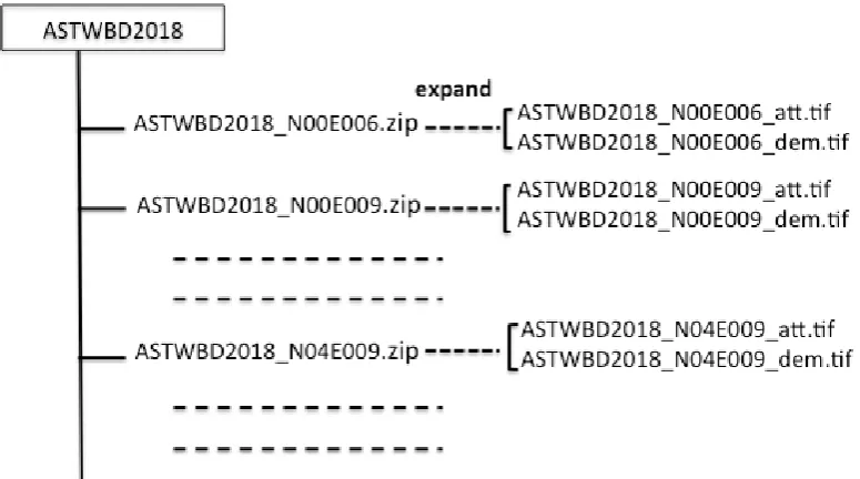
This paper describes how these improvements to the ASTER GWBD were accomplished. The new ASTER GWBD product consists of a global set of 1º latitude-by-1º longitude tiles that contain water body attribute and elevation data files in geographic latitude and longitude coordinates and with one arc-second postings. Consequently, each tile contains 3601-by-3601 data points, including one common column and one common row with its neighboring tiles. Figure 1 shows the ASTER GWBD folder structure, and Table 1 shows data format. Each tile is composed of an attribute file and a DEM file. The attribute file distinguish a type of waterbody; sea-waterbody (attribute 1), river-waterbody (attribute 2), and waterbody (attribute 3). The DEM file shows zero elevation for sea-waterbody, one unique (flattened) elevation for lake-waterbody, and stepwise elevation with a step of one meter for river elevation. In addition to ASTER GDEM V3, the improved ASTER GWBD also be released to public sometime in 2018

Table 1. DATA FORMAT

2. Sea-Waterbody

In order to set the elevation of sea-waterbodies to zero, they first must be separated from inland lakes and rivers. This separation was carried out for scene-based DEM generation using the global sea-waterbody database that was created using GTOPO30 [5, 15]. If the sea-waterbody area is larger than 80 % of the sea-waterbody database, this area is identified as a sea-waterbody. The 80% criterion was adopted to compensate for the inaccuracy of the database. The land-sea interface (sea shoreline) is determined during ASTER GDEM generation, by the ratio of the number of stacked-sea-waterbody data to the total number of stacked-pixel data. If the ratio is larger than 0.5, the pixel is assigned as a part of the sea waterbody. Otherwise, the pixel is considered to be land. The 50% criterion was adopted in consideration of tidal effects to present an average delineation [6].

In high latitude areas, another obstacle to accurate delineation of the sea shoreline is the presence of sea ice, whose effects must be removed if sea shorelines are to be accurately delineated in the ASTER GWBD and GDEM. Target areas for sea ice removal were selected using the global coarse mosaic image that was generated from

original ASTER GDEM data. A sea ice removal process was carried out for the following high latitude target areas:

1) Latitudes of 60 degrees north and further north areas 2) Latitudes of 60 degrees south and further south areas 3) Extreme south of Greenland

4) Hudson Bay 5) James Bay 6) Ungava Bay 7) Sea of Okhotsk 8) Bering Sea 9) Patagonia area

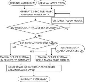
Figure 2 shows the algorithm flow for sea ice removal. It is difficult to delineate sea ice that occurs near sea shorelines using DEM data alone, because sea ice elevations frequently are similar to land elevations near the sea shoreline. Most sea ice exhibits elevations lower than 30 m, but land topography near sea shorelines often does not exceed 30 m, thus the possibility for confusion. Consequently, sea ice removal for the ASTER GWDB utilized ancillary data wherever useful data exist. Two such useful datasets were 1) the Canadian Digital Elevation Data (CDED) [17], which covers all of Canada with postings every 3 arc-seconds for latitude and every 3, 6, or 12 arc-seconds for longitude, depending on latitude; and 2) Alaska Digital Elevation Data [18] that covers the State of Alaska with postings every 2 arc-seconds of latitude and longitude. The processing steps employed in sea ice removal are summarized as follows:

1) Generate a 2° latitude-by-2° longitude tile mosaic from unimproved Version 3 ASTER GDEM data. 2) If the mosaic area includes any sea shoreline, continue the processing.

judgments, as necessary and possible.

4) The improved sea-waterbody data were incorporated into the ASTER GWBD. 5) Repeat step 1) to step 4) for all sea ice removal target areas.

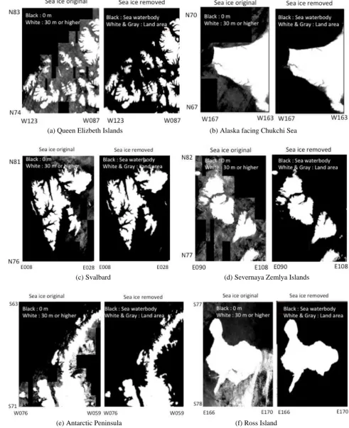
Figure 3 presents typical results from the sea ice removal process. Several examples are shown of original and corrected DEM images. Most, but not all, of the gray scale image areas shown in each first image of Figure 3 represent sea ice with elevations lower than 30 m. Some, however, are land areas that had to be identified and retained by manual intervention.

Figure 2 Algorithm flow for sea ice removal

3. Lake-Waterbody

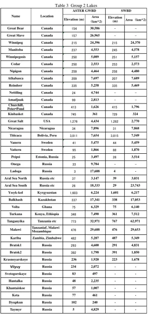
The main goal of lake-waterbody anomaly correction is to set the unique elevation value for each lake regardless of size. The lake grouping is needed because processing algorithm depends on the size of waterbodies. Lake-waterbodies are classified into three groups based on their size. Group1 lakes have sizes larger than a scene-based DEM. Table 2 lists seven lakes that belong to group1. Group2 lakes are lakes that are larger than a 2° latitude-by-2° longitude tiles mosaic image of ASTER GWBD and that do not belong to group1 lakes. Table 3 lists lakes belonging to group2. Group3 lakes are all lakes that do not belong to group1 or group2. Group3 lakes are expressed within a 2° latitude-by-2° longitude tiles mosaic image of ASTER GWBD data. The processing algorithm applied to any given lake depends on the waterbody group of that lake.

3.1. Processing Algorithm for Group1 Lake Waterbodies

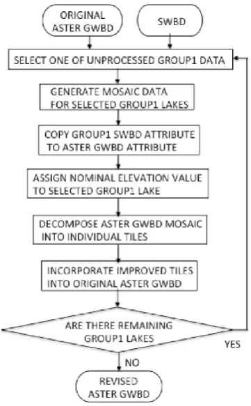
Group1 lakes all lie between 60°N latitude and 56° S latitude, so errors in the input ASTER GWBD covering these seven lakes can be corrected by replacing ASTER GWBD attributes with SWBD attributes. Figure 4 shows the algorithm flow for group1 lake anomaly correction. The process is carried out as follows:

1) Input original ASTER GWBD and SWBD. 2) Select one of the seven group1 lakes for correction.

3) Generate mosaic image data from both the input ASTER GWBD and the SWBD that cover the total area of the selected group1 lake.

(a) Queen Elizbeth Islands (b)Alaska facing Chukchi Sea

(c)Svalbard (d)Severnaya Zemlya Islands

(e)Antarctic Peninsula (f) Ross Island

Table 2 Grupe1 Lakes

Figure 4 Algorithm flow for group1 lake anomaly correction

5) Assign the nominal elevation value in Table 2 to the selected group1 lake. 6) Decompose the ASTER GWBD mosaic image data into individual tiles. 7) Incorporate the improved tiles into original input ASTER GWBD. 8) If uncorrected group1 lakes remain, repeat Step 2) to Step 7).

3.2. Processing Algorithm for Group2 Lake Waterbodies

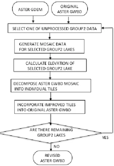
Group2 lake elevations were calculated using unimproved ASTER GDEM V3 data. The corrected elevation values for group2 lakes are reported in Table 3 and compared with corresponding SWBD lake elevation values, where available. Figure 5 shows the algorithm flow for correcting group2 lake elevations. The process is carried out as follows:

1) Input original ASTER GWBD and ASTER GDEM. 2) Select one of the group2 lakes for correction.

4) Calculate the elevation value of the selected lake surface by averaging perimeter elevations from the input ASTER GDEM data, using only the 10% of perimeter values that fall between 45% and 55% from the bottom in ascending order, since the perimeter elevations have the random errors, and the center value is close to real value without the random errors. The parameter 10% is empirically selected.

5) Decompose ASTER GWBD mosaic image data into individual tiles. 6) Incorporate the improved tiles into original input ASTER GWBD. 7) If uncorrected group2 lakes remain, repeat Step 2) to Step 6).

Figure 5 Algorithm flow for group2 lake elevation anomaly correction

3.3. Processing Algorithm for Group3 Lake Waterbodies

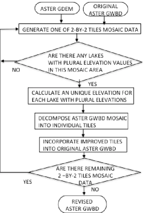
As mentioned previously, group3 lakes are expressed in 2° latitude-by-2° longitude tiles mosaics of ASTER GWBD and GDEM data created from 1° latitude-by-1° longitude tiles. Almost all lakes belong to group3. Most lakes within the original 1° latitude-by-1° longitude tiles were corrected during ASTER GDEM generation. However, some lakes may extend across adjacent tiles, regardless of the size. Thus, the lake elevations may be slightly different for the same lake connected through a tile boundary, such that they still exhibit plural elevations in the 2° latitude-by-2° longitude tiles mosaics. This type of anomaly must be corrected, so these lakes have one unique (flattened) elevation. Fig. 6 shows the algorithm flow for group3 lakes anomaly correction. The process is carried out as follows:

1) Input the unimproved Version 3 ASTER GWBD and ASTER GDEM.

2) Generate a 2° latitude-by-2° longitude tiles mosaic image data from both the input ASTER GWBD and the ASTER GDEM.

Figure 5 Algorithm flow for group2 lake elevation anomaly correction

3) If any lake in the mosaic area has plural elevations, go to next step to calculate the unique elevation for each abnormal lake. Otherwise, return to previous step 3) to generate the next mosaic image data.

4) Calculate the unique elevation value for each abnormal lake with plural elevations by averaging the perimeter elevation data. For averaging, use only the data between 45% and 55% from the bottom in ascending order by the same reason as the group2 lakes.

Table 3 Group 2 Lakes

Figure 6 Algorithm flow for group3 lake anomaly correction

4. River-Waterbody

River elevations are not constant, but rather gradually become lower from upstream to downstream. In order to assign rivers proper declining elevations, they first must be separated from lakes. Unfortunately, there is no automated way to achieve such separation. Consequently, in the initial stage of waterbody detection and assignment of elevation, all inland waterbodies are treated as lakes with a constant elevation value for each tile [5, 6]. The separation must be carried out by visual identification for each tile using the support tool. After separating rivers from lakes, river elevations are assigned stepwise elevations with a step of one meter. The stepwise elevation assignment is carried out by a manual or automated method, depending on the situation using the support program.

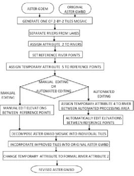
4.1. Basic Algorithm Flow for River Stepwise Elevation

Figure 7 shows the basic algorithm flow for determining river stepwise elevations. The process involves selecting a series of reference points along the course of a river and assigning those reference points unique elevations based on perimeter elevation values or based on SWBD data, where available. Reference point elevations must always step down (decrease) from upstream to downstream, and they must always be lower than their perimeter elevations. The process is carried out as follows:

1) Input original ASTER GWBD and ASTER GDEM.

2) Generate one of 2° latitude-by-2° longitude tiles mosaic image data from both the unimproved input ASTER GWBD and the ASTER GDEM.

5) Select river reference points from which stepwise elevations between adjacent reference points will be calculated by manual or automated editing, depending on the situation. Set reference point elevations based on perimeter data or SWBD data.

6) Temporarily designate river reference points as attribute 5.

7) Apply manual or automated editing to calculate stepwise elevations between adjacent reference points, using the support program.

8) Decompose ASTER GWBD mosaic image data into individual tiles. 9) Incorporate improved tiles into original input ASTER GWBD. 10) Change temporary attribute 5 to formal river attribute 2.

11) Repeat Step 2) to Step 10) for all land areas between latitudes 83°N and 83°S.

Figure 7 Basic algorithm flow for river stepwise elevation editing

4.2. Manual Stepwise Elevation Editing

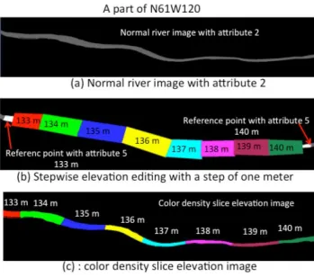
Figure 8 shows one example of manual stepwise elevation editing process. The process is very simple, and it usually is used in cases where the elevation difference between adjacent reference points is equal to or less than 16 meters, although this criterion can be flexibly changed depending on the situation. The process is carried out as follows.

1) Original river image for stepwise elevation editing is first masked for each elevation value as shown in Figure 8 (b) using the support tool. The elevation difference is roughly allocated in equal distance between adjacent reference points.

2) The attribute image area for each elevation value is selected by logical AND operation for each masked area and attribute 2 area.

4.3. Automated Stepwise Elevation Editing

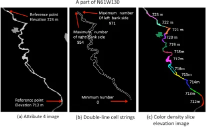
Figure 9 shows one example of the automated stepwise elevation editing process, which utilizes double-line cell strings to define stepwise river segments with decreasing elevations from upstream to downstream. Elevations for the stepwise river segments are calculated from the perimeter river bank elevations, as defined in the ASTER GDEM. Borderlines between connecting river segments are automatically defined and then adjusted to achieve the shortest path length between opposing shorelines. The process is carried out as follows:

1) Assign the river area between adjacent reference points as temporary attribute 4 to designate the automated stepwise elevation editing area, including the start point (Figure 9a).

2) Create double-line cell strings for the attribute 4 river segment from perimeter lines along the left and right river banks (Figure 9b). The perimeter string for the island in the river is excluded from the double-line cell strings, as shown in Fig. 9b.

3) Number each cell-string boundary line adjacent to the river from one reference point with the lowest elevation to the other reference points with the highest elevation. The starting minimum number is zero. The total numbers on the left bank side and right bank side may be slightly different, because the

two banks of the river do not have exactly the same shoreline distance between reference points.

4) Allocate consecutive cell string numbers for each one-meter step to calculate the borders at both bank sides and define

the stepwise river segments. Tentative borderlines on the river are connecting lines between two positions ( and

lines) at left and right banks as shown in Figure 10.

5) Rotate all border lines to have the shortest path lengths, since the borderlines with the shortest lengths are virtually at right angles to the river flow directions.

6) Assign the corresponding elevation values to all river sections between adjacent borders.

Figure 9(c) shows the final color density slice image of the newly defined stepwise river segments.

Figure 8 One example of manual editing process for river stepwise elevation.

Figure 9 One example of automated editing process for river stepwise elevation

Figure 10 Stepwise river elevation border line rotation to find Figure 11 Algorithm flow to incorporate ASTER GWBD shortest length. data into ASTER GDEM

5. Incorporation of Waterbody Data into GDEM

ASTER GWBD folders include two files: an attribute file and a DEM file, as shown in Fig. 1. The improved waterbody elevation data, based on previous sections, are described in the DEM files, and must be incorporated into ASTER GDEM to reflect the improved results. At the same time, it is essential to keep the consistency between waterbodies and their perimeter elevation values. The perimeter elevations must be higher than the waterbody elevation. Figure 11 shows the algorithm flow to incorporate ASTER GWBD data into ASTER GDEM. The process is carried out as follows:

1) Input original Version 3 ASTER GDEM and the now improved ASTER GWBD. 2) Select one ASTER GWBD tile and the corresponding original ASTER GDEM tile. 3) Copy the waterbody elevation data into the original ASTER GDEM tile.

4) Edit the land elevations along sea shorelines such that those are equal to or higher than one meter.

5) Edit the perimeter elevations for all lakes in the tile such that those are at least one meter higher than the lake elevation values.

6) Edit the perimeter elevations for all one-meter steps of rivers in the tile such that those are at least one meter higher than the elevations of the one-meter step area.

7) Repeat Step 2) to Step 6) for all ASTER GWBD tiles.

Typical examples of the final improved results are shown in Figures12 to 14. These shaded-relief images clearly show that all sea and lake waterbodies are completely flattened regardless of their sizes. For river-waterbodies, each stepwise elevation area is flattened, as shown in Figure14.

6. Summary

A waterbody detection technique is an essential part of DEM generation to delineate land-water boundaries and to set flattened elevations. This paper described the technical methodology for improving the initial tile-based waterbody data that are created during generation of the ASTER GDEM, but which are not suitable for incorporating into new ASTER GDEM Version 3. Waterbodies are classified into three categories: sea, lake, and river.

Sea-waterbodies were separated from inland waterbodies, and their elevations were set to zero. The effects of sea ice were removed to better delineate sea shorelines in high latitude areas, because sea ice prevents accurate delineation of sea shorelines. This process was enhanced by reference to ancillary data, specifically Google Earth and GeoCover images.

Lake waterbodies are classified into three groups based on size. Group1 lakes are much larger than scene DEMs, which thus do not include enough land area to define the lake or calculate its elevation. For Group1 lakes the corresponding SWBD attribute image was used to define the ASTER GWBD area, and the nominal elevation value was used to assign the lake elevation. Group2 lakes have a size larger than a 2° latitude-by-2° longitude tiles mosaic image of ASTER GDEM data and do not belong to group1 lakes. Group3 lakes are all other lakes. For group2 and group3 lakes, the elevation for each lake was calculated from the perimeter elevation data using the mosaic image that covers entire area of the lake.

River elevations are not constant but gradually decline from upstream to downstream. Rivers were separated from lakes by visual inspection, because there is no automated way to discriminate between rivers and lakes. A stepwise elevation assignment was carried out for rivers using manual or automated methods, depending on the situation under support program.

All improved waterbody elevation data were incorporated into the ASTER GDEM Version 3 to reflect the improved results. At the same time, the waterbody perimeter elevations were edited such that those were at least one meter higher than the waterbody elevation.

(a) Attribute image of Great Lakes (b) Shaded-relief elevation image of Great Lakes green denotes lake, red denotes river

Figure 12 Final improved images of Great Lakes.

(a) Attribute image of Great Slave Lake (b) Shaded-relief elevation image of Great Slave Lake green denotes lake, red denotes river

Figure 13 Final improved images of Great Slave Lake.

(a) Attribute image of Coronation Gulf area, (b) Shaded-relief elevation image of Coronation Gulf area blue denotes sea, red denotes river, green denotes lake.

References

1. H. Fujisada, F. Sakuma, A. Ono, and M. Kudo, Design and preflight performance of ASTER instrument protoflight model, IEEE Transactions on Geoscience and Remote Sensing, vol.36, no.4, pp.1152-1160, 1999.

2. H. Fujisada, “ASTER Level-1 data processing algorithm,” IEEE Transactions on Geoscience and Remote Sensing, vol.36, no.4, pp.1101-1112, 1998.

3. H. Fujisada, G. B, Bailey, G. G. Kelly S. Hara, and M. Abrams, ASTER DEM performance, IEEE Transactions on Geoscience and Remote Sensing, vol.43, no.12, pp.2707-2714, 2005.

4. Fujisada, A. Iwasaki, and S. Hara, ASTER stereo system performance, Proc. SPIE Vol.4540, pp.39-49, 2001 Toulouse.

5. H. Fujisada, M. Urai, and A. Iwasaki, Advanced methodology for ASTER DEM generation, ‘’IEEE Transactions on Geoscience and Remote Sensing, vol.49, no.12, pp.5080-5091, 2011.

6. H. Fujisada, M. Urai, and A. Iwasaki, Technical methodology for ASTER global DEM, IEEE Transactions on Geoscience and Remote Sensing, vol.50, no.10, pp.3725-3736, 2012.

7. M. L. Carroll, J. R. Townshend, C. M. DiMiceli, P. Noojipady, and R. A. Sohlberg, A new global raster water mask at 250 m resolution, 8. M. Feng, J. O. Sexton, S. Channan, and J. R. Townshend, A global, high-resolution (30-m) inland water body dataset for 2000 : first

results of a topographic–spectral classification algorithm, International Journal of Digital Earth, 2015. http://dx.doi.org/10.1080/17538947.2015.1026420

9. C. Verpoorter, T. Kutser, D. A. Seekell, and L. J. Tranvik, A global inventory of lakes based on high-resolution satellite imagery Geophys. Res. Lett., 41, 6396–6402, doi:10.1002/2014GL060641.

10. C. Verpoorter, T. Kutser, and L. Tranvik, Automated mapping of water bodies using Landsat multispectral data, Limnol. Oceanogr.: Methods 10, 2012, 1037–1050 © 2012, by the American Society of Limnology and Oceanography, Inc.

11. JeanFrançois Pekel, Andrew Cottam, Noel Gorelick and Alan S. Belward , High-resolution mapping of global surface water and its longterm changes, Nature vol.540, No.7633, pp418-422, 2016.

12. SRTM Data Editing Rules, Version 2.0, 2003 https://dds.cr.usgs.gov/srtm/version2_1/Documentation/SRTM_edit_rules.pdf 13. SRTM Water Body Data Product Specific Guidance, Version 2.0, 2003”

https://dds.cr.usgs.gov/srtm/version2_1/SWBD/SWBD_Documentation/SWDB_Product_Specific_Guidance.pdf

14. James A. Slater and James Little, “The SRTM Data Finishing Process and Products”, Photogrammetric Engineering & Remote Sensing, vol.72, no.3, 2006.

15. GTOPO30

https://lta.cr.usgs.gov/GTOPO30

16. LandsatGeocoverMosaics http://glcf.umd.edu/data/mosaic/ 17. Canada digital elevation data

https://uwaterloo.ca/library/geospatial/collections/canadian-geospatial-data-resources/canada/canada-digital-elevation-data-cded [18] Alaska Digital Elevation Models