Neural Frequency Sweeper for Accelerating S-Parameters Calculation of Planar Microwave Structures

(1)

NEURAL FREQUENCY SWEEPER FOR

ACCELERATING S-PARAMETERS CALCULATION OF PLANAR MICROWAVE STRUCTURES

E. A. Soliman

Physics Department

School of Sciences and Engineering The American University in Cairo P. O. Box 2511, Cairo 11511, Egypt

M. S. Ibrahim

Department of Engineering Physics and Mathematics Faculty of Engineering

Cairo University Giza 12211, Egypt

Abstract—This paper presents a new frequency-sweep approach for the eﬃcient calculation of S-parameters of planar microwave structures. The approach is based on approximating the frequency dependence of the real and imaginary parts of the S-parameters using neural networks. Due to its superior performance, radial basis functions neural network (RBF-NN) is adopted. A limited number of frequency samples are used to train the RBF-NN. Then, the trained RBF-NN is capable of providing a smooth frequency response with very high accuracy in a fraction of a second. The proposed method is applied to a number of planar microwave structures such as: Patch antenna with an inset feed, band-rejection ﬁlter, and branch-line coupler. According to the presented results, a speed factor of at least 10 is measured, and a maximum percentage error of 3.29% is recorded.

1. INTRODUCTION

(2)

modifying the strengths of the connections during a learning phase [1]. Ability and adaptability to learn, generalisability, fast real-time operation, and ease of implementation have made NNs popular for a number of microwave design problems in recent years [2]. Citing just a number of examples: NNs have been used in the design of passive microwave circuits [3], analysis and synthesis of microstrip lines [4], calculation of the characteristic impedance of air-suspended trapezoidal and rectangular-shaped microshield lines [5], design of nonlinear microwave circuits based on active devices [6], design of microstrip patch antennas [7, 8], direction of arrival estimation with antenna arrays [9, 10], radar target recognition [11], aperture antenna shape prediction [12], inverse scattering of dielectric cylinders [13], near ﬁeld to far ﬁled transformation [14], and synthesis of antenna array [15, 16]. In addition to modeling the response, NNs can also be employed within the core of the full-wave solvers based on the method of moments [17, 18].

In this work neural networks are employed to accelerate the frequency sweep required by full-wave simulators for calculating the

S-parameters of microwave devices. There are several techniques that can be used for this purpose. These techniques can be classified into three main categories. In the first category, the frequency response, such as an S-parameter, is approximated using Padé approximant. Several techniques can be used to achieve this task such as MBPE, AWE, CFH, and PVL [19]. The basic principle of these techniques is to extract the dominant poles and residues of the frequency response and represent it by a reduced-order model.

The second main category is the impedance matrix interpolation technique. This technique is based on the fact that most responses of interest, such as the current distribution and theS-parameters, exhibit rapid frequency variations. However, the impedance matrix elements are smoother in their variation with frequency. Consequently, it is better to frequency interpolate them rather than trying to interpolate the responses. The concept of the impedance matrix interpolation was proposed in [20]. The approach is further extended in [21]. These works are concerned with the analysis of structures in free space. A similar technique is presented in [22], which is suitable for planar structures in layered media.

(3)

frequency point.

The technique presented in this paper belongs to the ﬁrst category. A neural network is trained to approximate the S-parameters at any frequency point. A limited number of frequency samples are used to train such neural network. Once trained, this neural network is capable of performing the frequency sweep in a fraction of a second. Section 2presents the proposed frequency sweeper based on radial basis functions neural networks. This frequency sweeper has been used for rapidly calculating the S-parameters of a number of microwave structures in Section 3. The important conclusions are stated in Section 4.

2. NEURAL FREQUENCY SWEEPER

The remarkable ability of radial basis function neural networks (RBF-NN) to carry out general nonlinear function approximation tasks through learning from examples is exploited in this research. RBF-NN posses several advantages over the most commonly used back propagation neural network (NN). RBF-NN trains faster than BP-NN. Moreover RBF-NN leads to better decision boundaries in a variety of applications.

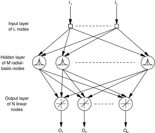
Radial basis function neural network is composed of three layers called input, hidden, and output layers as shown in Fig. 1. The input layer is made up of L nodes, where L is the dimension of the input vector. The task of the input layer is to pass the inputs of the network to the hidden layer. The hidden layer in turn performs a nonlinear mapping from the input space to a new space. It is made up of M

nodes, each with a radial activation function. The most common choice for this function is the Gaussian function which has a peak at the center and decreases monotonically as the distance from the center increases. The region of the input space over which the node has an appreciable response, is known as the “spread”. It is important that the spread should be large enough to enable the hidden nodes to respond to overlapping regions of the input space, but not so large that all the hidden nodes respond in the same manner. The output layer is made up of N linear nodes which are fully connected to the hidden nodes. Therefore the output nodes form a linear combination of the outputs of the hidden nodes.

(4)

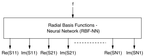
the least mean squares algorithm for training in the output layer. Figure 2shows the topology of the proposed frequency-sweeper which is based on radial basis functions neural network. The proposed RBF-NN takes the frequency as an input and predicts the real and imaginary parts of all S-parameters of interest. A number of frequency samples are selected within the frequency band of interest.

S-parameters of the microwave structure under investigation are calculateda prior at the selected frequency samples. The combination of frequency points (inputs) and the corresponding S-parameters (outputs) are known as patterns. These patterns are divided into two interlaced parts. The ﬁrst part is used to train the frequency-sweeper, while the second part is used to test it.

Input layer of L nodes

Hidden layer of M radial-basis nodes

Output layer of N linear

nodes

I1

O₁ O₂ O_N

IL

Figure 1. Radial basis functions neural network (RBF-NN).

Although the magnitude of an S-parameter on the dB scale, is usually of more interest than its real and imaginary parts, the latter show smoother behavior. The former always possesses sharp variations around resonance frequency [17, 23]. For this reason, it is much more eﬃcient to model the real and imaginary parts rather than the magnitude on the dB scale. Then, the dB value can be very easy calculated in terms of the real and imaginary parts: S(dB) = 20 log₁₀

Re2(S) + Im2(S)

(5)

Re(S11)

Radial Basis Functions - Neural Network (RBF-NN)

f

Im(S11) Re(S21) Im(S21) Re(SN1) Im(SN1)

Figure 2. Topology of the proposed frequency sweeper based on RBF-NN.

3. APPLICATIONS

In this section, the proposed frequency sweeper is applied to three planar microwave structures: Patch antenna with an inset feed, band-rejection ﬁlter, and branch-line coupler. All these structures are assumed made of perfect conductor on top of a Duroid substrate with dielectric constant of 2.2 and thickness of 0.794 mm, backed with a perfect conductor ground plane. The preparation of the training and testing patterns is carried out using ADS/Momentum [26]. Momentum is a 2.5D full-wave solver based on the integral equation formulation solved using the method of moments. For meshing the microwave structures under investigation, mixed rectangular and triangular segments are used. Twenty cells per wavelength combined with a narrow edge mesh are adopted.

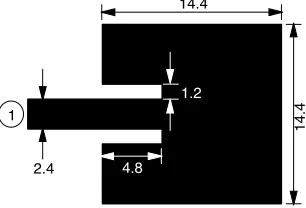
3.1. Patch Antenna with an Inset

(6)

14.4

14.

4

2.4 4.8

1.2

1

Figure 3. Patch antenna with an inset feed (all dimensions are in mm).

6.5 6.6 6.7 6.8 6.9 7 7.1 7.2 7.3 7.4 7.5

-1.2 -0.9 -0.6 -0.3 0 0.3 0.6 0.9 1.2

Re (Exact) Re (RBF-NN) Im (Exact) Im (RBF-NN)

Frequency (GHz)

S11

Figure 4. Re(S11) and Im(S11) of the patch antenna versus frequency

as obtained using the exact simulator and the RBF-NN model.

The time required by the trained RBF-NN to calculate 201 points is 41.9 msec. Hence the total time required to obtain these 201 points using RBF-NN is: Time required to prepare 13 training points (46.57 sec) + time required for training (46.7 msec) + time required for sweeping (41.9 msec) = 46.66 sec. To calculate the same 201 points using ADS/Momentum, 12minutes are required. This means that the proposed frequency sweeper is about 15.43 times faster.

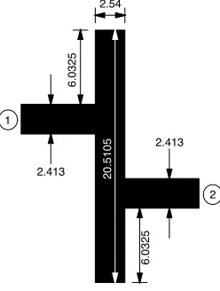
3.2. Band-rejection Filter

(7)

2.54

2.413

6.0325

20.5105

1

2

Figure 5. Band-rejection ﬁlter (all dimensions are in mm).

3 4 5 6 7 8 9 10 11

-0.9 -0.6 -0.3 0 0.3 0.6 0.9 1.2 1.5

Frequency (GHz)

S1

1

Figure 6. Re(S11) and Im(S11) of the band-rejection ﬁlter versus frequency as obtained using the exact simulator and the RBF-NN model.

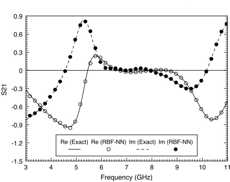
symmetry of the two ports of this ﬁlter, S11=S22. From reciprocity, S21=S12. Hence, this ﬁlter is characterized by only two independent S-parameters: S11 and S21. The real and imaginary parts of these

parameters are the outputs of the RBF-NN of this ﬁlter. Figs. 6 and 7 show S11 and S21, respectively, as obtained using RBF-NN

(8)

3 4 5 6 7 8 9 10 11 -1.5

-1.2 -0.9 -0.6 -0.3 0 0.3 0.6 0.9

Frequency (GHz)

S2

1

Figure 7. Re(S21) and Im(S21) of the band-rejection ﬁlter versus

frequency as obtained using the exact simulator and the RBF-NN model.

Re (S11), Im (S11), Re (S21), and Im (S21) are 2.78%, 2.51%, −2.35%,

and −2.23%, respectively. For training the RBF-NN of this ﬁlter, 20 frequency samples are used. It has 16 neurons in the hidden layer.

The proposed RBF-NN model requires a total time of 124.53 sec to produce 201 frequency points. This time can be distributed as follows: Time required to prepare 20 training points using ADS/Momentum (124.48 sec) + time required for training (49.1 msec) + time required for sweeping (4.91 msec) = 124.53 sec. To calculate the same 201 points using the full-wave simulator, 20.85 minutes are required. Hence the proposed frequency sweeper oﬀers a speed factor of about 10.

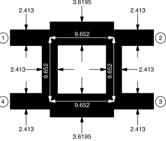
3.3. Branch-line Coupler

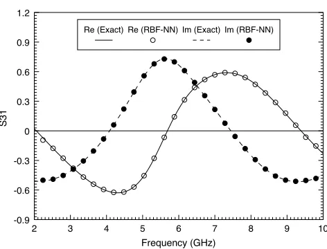
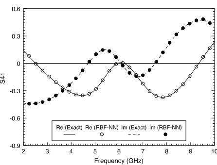
The last example is a branch-line coupler, as shown in Fig. 8. This coupler has 4 ports and characterized by 16 S-parameters. Due to symmetry and reciprocity, only four S-parameters are independent, namely S11, S21, S31, and S41. The RBF-NN frequency sweeper of

Fig. 2is applied to this coupler. For training the associated RBF-NN, 15 frequency samples are used. The trained RBF-NN has 11 neurons in its hidden layers. For testing this RBF-NN, another 30 points, uniformly distributed along the frequency band of interest, are used. Figs. 9, 10, 11, and 12show the exact and the RBF-NN results ofS11, S21,S31, andS41, respectively. Again, both methods lead to very close

(9)

2.413

2.413 2.413

2.413

3.6195

2.413 2.413

9.652

9.65

2

9.652

1 2

4 3

Figure 8. Branch-line coupler (all dimensions are in mm).

2 3 4 5 6 7 8 9 10

-0.6 -0.3 0 0.3 0.6 0.9 1.2

Frequency (GHz)

S11

Figure 9. Re(S11) and Im(S11) of the branch-line coupler versus frequency as obtained using the exact simulator and the RBF-NN model.

Im (S11), Re (S21), Im (S21), Re (S31), Im (S31), Re (S41), and Im (S41)

are 3.05%, −2.10%, 2.61%, 3.29%, 3.09%, 1.78%, 1.03%, and 2.84%, respectively.

(10)

2 3 4 5 6 7 8 9 10 -1.2

-0.9 -0.6 -0.3 0 0.3 0.6 0.9

Frequency (GHz)

S21

Figure 10. Re(S21) and Im(S21) of the branch-line coupler versus frequency as obtained using the exact simulator and the RBF-NN model.

2 3 4 5 6 7 8 9 10

-0.9 -0.6 -0.3 0 0.3 0.6 0.9 1.2

Frequency (GHz)

S31

Figure 11. Re(S31) and Im(S31) of the branch-line coupler versus

(11)

2 3 4 5 6 7 8 9 10 -0.9

-0.6 -0.3 0 0.3 0.6

Frequency (GHz)

S41

Figure 12. Re(S41) and Im(S41) of the branch-line coupler versus

frequency as obtained using the exact simulator and the RBF-NN model.

4. CONCLUSION

A new RBF-NN model is presented in this paper. The model takes the frequency as an input and provides the real and imaginary parts of the S-parameters as outputs. Such model can be used to perform the frequency sweep required for characterizing a planar microwave structure. A limited number of frequency points uniformly distributed along the frequency band of interest, are used to train the RBF-NN frequency sweeper. The presented results demonstrate that the trained RBF-NN performs the frequency sweep very fast and with very high accuracy. For the examples studied in this paper, the maximum recorded percentage error in the prediction of the real and imaginary parts of S-parameters is 3.29%. For these examples, the RBF-NN sweeper is at least 10 times faster than the full-wave simulator. The proposed method is quite general and can be applied to any planar microwave structure.

REFERENCES

1. Maren, A., C. Harston, and R. Pap, Handbook of Neural Computing Applications, Academic Press, 1990.

(12)

3. Watson, P. and K. C. Gupta, “EM-ANN models for microstrip vias and interconnects in dataset circuits,” IEEE Trans. Microwave Theory Tech., Vol. 44, 2495–2503, Dec. 1996.

4. Soliman, E. A., M. H. Bakr, and N. K. Nikolova, “Modeling of microstrip lines using neural networks — Applications to the design and analysis of distributed microstrip circuits,”Int. J. RF

and Microwave Computer-Aided Eng., Vol. 14, 166–173, March

2004.

5. Guney, K., C. Yildiz, S. Kays, and M. Turkmen, “Artiﬁcial neural networks for calculating the characteristic impedance of air-suspended trapezoidal and rectangular-shaped microshield lines,”

Journal of Electromagnetic Waves and Applications, Vol. 20,

1161–1174, 2006.

6. Zaabab, A. H., Q.-J. Zhang, and M. Nakhla, “A neural network approach to circuit optimization and statistical design,” IEEE Trans. Microwave Theory Tech., Vol. 43, 1349–1358, June 1995. 7. Mishra, R. K. and A. Patnaik, “Neural network-based CAD model

for the design of square-patch antennas,”IEEE Trans. Antennas Propagat., Vol. 46, 1890–1891, Dec. 1998.

8. Mohamed, M. D. A., E. A. Soliman, and M. A. El-Gamal, “Optimization and characterization of electromagnetically coupled patch antennas using RBF neural networks,” Journal of Electromagnetic Waves and Applications, Vol. 20, 1101–1114, 2006.

9. El-Zooghby, A. H., C. G. Christodoulou, and M. Georgiopoulos, “Performance of radial basis function networks for direction of arrival estimation with antenna array,” IEEE Trans. Antennas Propagat., Vol. 45, 1611–1617, Nov. 1997.

10. Zainud-Deen, S. H., H. A. Malhat, K. H. Awadalla, and E. S. El-Hadad, “Direction of arrival and state of polarization estimation using radial basis function neural network (RBFNN),” Progress In Electromagnetics Research B, Vol. 2, 137–150, 2008.

11. Zhao, Q. and Z. Bao, “Radar target recognition using a radial basis function,”Neural Networks, Vol. 9, 709–720, April 1996. 12. Washington, G., “Aperture antenna shape prediction by feed

forward neural networks,” IEEE Trans. Antennas Propagat., Vol. 45, 683–688, April 1997.

(13)

14. Ayestarán, R. G. and F. Las-Heras, “Near field to far field transformation using neural networks and source reconstruction,”

2201–2213, 2006.

15. Ayestar´an, R. G., J. Laviada, and F. Las-Heras, “Synthesis of passive-dipole arrays with a genetic-neural hybrid method,”

2123–2135, 2006.

16. Ayestar´an, R. G., F. Las-Heras, and J. A. Martinez, “Non uniform-antenna array synthesis using neural networks,” Journal of Electromagnetic Waves and Appls, Vol. 21, 1001–1011, 2007. 17. Soliman, E. A., M. H. Bakr, and N. K. Nikolova, “Neural

Networks — Method of Moments (NN-MoM) for the eﬃcient ﬁlling of the coupling matrix,” IEEE Transactions on Antennas and Propagation, Vol. 52, 1521–1529, June 2004.

18. Soliman, E. A., M. A. El-Gamal, and A. K. Abdelmageed, “Neural network model for the eﬃcient calculation of Green’s functions in layered media,” International Journal of RF and Microwave Computer-Aided Engineering, Vol. 13, 128–135, March 2003. 19. Ling, F., D. Jiao, and J.-M. Jin, “Eﬃcient electromagnetic

modeling of microstrip structures in multilayer media,” IEEE Trans. Microwave Theory Tech., Vol. 47, 1810–1818, Sept. 1999. 20. Newman, E. H., “Generation of wide-band data from the method

of moments by interpolating the impedance matrix,”IEEE Trans. Antennas Propagat., Vol. 36, 1820–1824, Dec. 1988.

21. Virga, K. and Y. Rahmat-Samii, “Eﬃcient wide-band evaluation of mobile communications antennas using [Z] or [Y] matrix interpolation with the method of moments,” IEEE Trans. Antennas Propagat., Vol. 47, 65–76, Jan. 1999.

22. Yeo, J. and R. Mittra, “An algorithm for interpolating the frequency variations of method-of-moments matrices arising in the analysis of planar microstrip structures,”IEEE Trans. Microwave Theory Tech., Vol. 51, 1018–1025, March 2003.

23. Soliman, E. A., “Rapid frequency sweep technique for MoM planar solvers,” IEE Proceedings Microwaves, Antennas & Propagation, Vol. 151, 277–282, Aug. 2004.

24. MATLAB, version 7.0, The MathWorks Inc., 2004.

25. Jokinen, P. A., “Neural networks with dynamic capacity allocation and quadratic function neurons,” Proc. of NEURO-Nimes 90, Nimes, France, 1990.