A Novel Non-Homogeneous STAP Algorithm for Target-Like Signal Elimination Based on Sparse Reconstruction

A Novel Non-Homogeneous STAP Algorithm for Target-Like Signal

Elimination Based on Sparse Reconstruction

Qi Zhang1, *, Mingwei Shen1, Jianfeng Li1, Di Wu2, and Daiyin Zhu2

Abstract—Space-time adaptive processing (STAP) for airborne radar employs training samples to estimate clutter covariance matrix (CCM). However, the target-like signals contained in the training samples severely corrupt the accuracy of the CCM. This paper proposes a novel non-homogeneous STAP algorithm for target-like signal elimination based on reduced-dimension sparse reconstruction (RDSR) to overcome this issue. The proposed algorithm exploits the high-resolution angle-Doppler spectrum obtained by RDSR to estimate and eliminate target-like signals. Theoretical analysis and simulation results show that the proposed algorithm effectively suppresses clutter and improves the performance of STAP in non-homogeneous environments.

1. INTRODUCTION

Airborne radar has been applied in ground motive target detection extensively. However, the relative speed and extending Doppler frequency of the clutter caused by the platform motion lead to seriously performance degradation of the target detection. Spacetime adaptive processing (STAP) is an important tool for clutter suppression in the advanced airborne radar system [1, 2]. The conventional STAP algorithm employs training samples to estimate the clutter covariance matrix (CCM). According to the theory of STAP [3], if the CCM is estimated accurately, the training samples should be independent and identically distributed (IID), and the number of IID samples must be twice as many as the system degrees of freedom (DOFs).

However, the actual non-homogeneous clutter environments result in poor accuracy of CCM estimation [4], which affects the target extraction severely. In the last few years, the problems of adaptive radar detection and clutter suppression in nonhomogeneous environments are thoroughly researched [5– 7]. In order to improve the performance of target detection in heterogeneous environments, training data selection techniques have been proposed, such as generalized inner product (GIP) algorithm [8, 9], adaptive power residue (APR) algorithm [10], power-selected training (PST) algorithm [11] and training sample selection algorithm based on the similarity between the cell under test (CUT) and training samples [12, 13]. However, in the extremely nonhomogeneous environments with dense distribution of target-like signals (for example, over the city or on the highway), conventional training data selection algorithms will lead to significant reduction of the sample size, which increases the estimation error of CCM.

Recently, the sparse recovery (SR) technique has been applied to STAP. SR-STAP algorithms [14– 18] utilize the clutter sparse property in the angle-Doppler plane and recover complex amplitudes of clutter scatterers by means of SR theory [19, 20]. Compared with conventional STAP algorithms, SR-STAP algorithms can be more accurate with fewer training snapshots. In this paper, we propose a target-like signal elimination algorithm based on reduced-dimension sparse reconstruction (RDSR). Firstly, the proposed algorithm employs RDSR to obtain high-resolution angle-Doppler spectrum.

Received 10 May 2018, Accepted 13 August 2018, Scheduled 27 August 2018 * Corresponding author: Qi Zhang (15950552066@163.com).

Subsequently we use the angle-Doppler spectrum to implement high-precision estimation on the spatial frequency, Doppler frequency and amplitude of the target-like signal and then subtract the target-like signal from the training sample. Simulation results confirm the effectiveness of the proposed algorithm in nonhomogeneous environments. The main contributions are summarized as follows:

1. Compared to the conventional NHD algorithms rejecting nonhomogeneous training samples directly, the proposed method subtracts target-like signals from training samples, which makes the training samples reapplied to the STAP weight calculation, avoiding the drastic reduction of the sample size when target-like signals are densely distributed, effectively improving the accuracy of CCM estimation.

2. We analyse the maximum error of the target-like signal elimination algorithm and present a novel high-precision algorithm. The simulation results show that the novel algorithm can accurately eliminate the target-like signal and improve the target detection performance of the STAP system. 3. In addition, in order to improve the operational efficiency, we use the main beam detection to detect training samples contaminated by target-like signals and use the improved OMP algorithm to obtain the angle-Doppler spectrum.

The remainder of this paper is organised as follows: Section 2 gives the principle of target-like signal elimination algorithm. Aiming at the estimation error of the target-like signal, a high-precision estimation algorithm based on RDSR is proposed in Section 3. Section 4 is devoted to the simulation results and performance analyses. Finally, the conclusions are given in Section 5.

Notations: In this paper, the operations of transposition and conjugate transposition are expressed by superscripts [·]T and (·)H, respectively. The symbol ⊗ denotes the Kronecker product. · indicates the spot product. arg min

x

g(x) represents the value of x when the g(x) is minimum. x₁ and x₂

denote l1-norm andl2-norm operations ofx.

2. THE PRINCIPLE OF TARGET-LIKE SIGNAL ELIMINATION

Consider a non-side looking pulsed-Doppler radar system (i.e., There is a certain angulation between the array axis and the flight direction) on an airborne platform. The radar antenna is a uniform linear array (ULA) consisting ofN elements with a fixed element distanceλ/2, where λis the wavelength of radar. In every coherent processing interval (CPI), the radar transmitsK coherent pulses with a pulse repetition frequencyf_r. Suppose that thelth range cell contains the target-like signal, the received data of the lth range cell X_l is given by

X_l =X_C +X_I+N_l (1) whereX_C denotes the clutter signal,X_I the target-like signal, and N_l the received noise.

2.1. Angle-Doppler Spectrum Estimation Based on RDSR

For notational convenience, the received signal X_l can be reshaped into a N×K matrix as

X_l = [S_l1Sl2 . . . Sl K]N×K (2) where S_{l i} represents the spatial snapshot vector from the N element array for the ith pulse of a K

pulse CPI. In order to limit the sidelobe level in the Doppler domain, we process the received signal by adding windows, and the windowed signal can be described by

T X_l =X_l·T_w= [S_T 1 ST 2 . . . ST K]N×K (3) where S_{T i} is the windowed spatial snapshot vector from theN element array for theith pulse of aK

pulse CPI. T_w denotes the window matrix whose structure is formulated as

T_w= ⎡ ⎢ ⎢ ⎣

w(1)

w(2) . . .

w(K) ⎤ ⎥ ⎥ ⎦

K×K

wherew(n)(n= 1,2,3, . . . , K) denote the window function coefficients. The data in the spatial-temporal domain can be transformed to the element-Doppler domain via one-dimensional Fourier Transform, which can be implemented as

D X_l=T X_l·F_D = [S_D1 SD2 . . . SD K]N×K (5) whereF_D denotes the Fast Fourier Transform (FFT) matrix, andS_{D i} represents the element-Doppler vector corresponding to the ith Doppler cell.

We discretize the spatial angle intoN_s=γN resolution cells, and the parameterγ is the resolution scale. The spatial angleθ_p and spatial frequencyf_spof thepth resolution cell are, respectively, expressed by

θ_p = 2π(p−1)

N_s (6)

f_sp = d

λcosθp (7)

then the spatial steering vector of thepth resolution cell is given by

φ_p = [1, exp(j2πf_sp), exp(j2πf_sp·2), . . . , exp(j2πf_sp·(N −1))]T (8) and the spatial steering dictionary ψ_i is formulated as:

ψ_i= [φ1, φ2, . . . , φNs]N×Ns (9)

both the target-like signal and clutter responses in the angle domain can be computed as follows:

ˆ

σ_i = arg min

σi

σ_i1

s.t.S_{D i}−ψ_iσ_i2 ≤ε_i (10)

where ˆσ_i is the estimated spatial distribution of target-like signal and clutter within theith Doppler cell, and ε_i is the error allowance. Equation (10) can be solved via improved orthogonal matching pursuit (OMP) [21]. Applying this procedure repeatedly for all Doppler cells, the angle-Doppler spectrum of both target-like signal and clutter can be obtained.

2.2. Estimation and Elimination of the Target-Like Signal

Suppose that the maximum pixel coordinate of the target-like signal on the angle-Doppler spectrum is (K_s, K_d) and that corresponding amplitude is a. According to the spatial steering dictionary we constructed, the estimated spatial frequency of the target-like signal is given by

f_{s E} = d

λcos

2π(K_s−1)

N_s

(11)

Because of the properties of FFT transformation, the estimated normalized Doppler frequency of the target-like signal can be expressed as

f_{d E} =−0.5 + 1

K(Kd−1)

(12)

Using recovery coefficientw= K

n=1

w(n)/K to calibrate windowing effect, the maximum pixel amplitude

of the target-like signal after correction is

a0=a/w (13)

Since FFT transform leads to the coherent accumulation of the signal amplitude in the frequency domain, the estimated amplitude is

α_E =a0/K (14)

Thus the estimated target-like signal is expressed as

whereS_{s E} and S_{d E} are the estimated spatial and temporal steering vector, which are defined by

S_{s E} = [1 exp(j2πf_{s E}) exp(j2πf_{s E}·2) . . . exp(j2πf_{s E}·(N −1))]T (16)

S_{d E} = [1 exp(j2πf_{d E}) exp(j2πf_{d E}·2) . . . exp(j2πf_{d E}·(K−1))]T (17) Subtracting the estimated target-like signal from the received signalX_l, the sample without target-like signalX_f can be computed as:

X_f =X_l−X_E (18)

The numerical simulations are carried out to validate the performance of the proposed algorithm and the main parameters of the simulated data are listed in Table 1.

Table 1. Parameters for simulation.

Parameters Value

Pulse Repetition Frequency (PRF) 5000 Hz

Bandwidth 5 MHz

Platform Velocity 130 m/s

Platform Height 8000 m

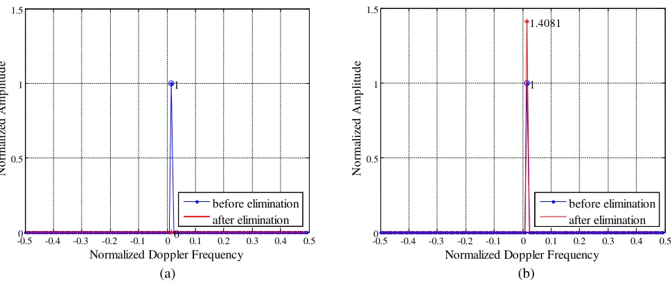
For instance, givenN = 16, K= 128 andγ = 8, we insert a target-like signal at the azimuth angle of 0◦, which is aligned with the main beam direction, and its signal-to-clutter-plus-noise ratio (SCNR) is set to −10 dB. Fig. 1 shows the angle-Doppler spectrum of target-like signal and clutter. Due to the coupling relationship between spatial frequency and Doppler frequency, clutter components are mainly distributed along the clutter ridge. Pixel point separated from the clutter ridge is the target-like signal that we are going to eliminate.

Figure 1. Angle-Doppler spectrum using RDSR based on improved OMP.

-0.50 -0.4 -0.3 -0.2 -0.1 0 0.1 0.2 0.3 0.4 0.5 0.5

1 1.5

Normalized Doppler Frequency

N o rm aliz ed A m p litu d e 1 0 before elimination after elimination

-0.50 -0.4 -0.3 -0.2 -0.1 0 0.1 0.2 0.3 0.4 0.5 0.5

1 1.5

Normalized Doppler Frequency

N o rm aliz ed A m p litu d e 1 1.4081 before elimination after elimination (b) (a)

Figure 2. The normalized amplitude of the target-like signal before and after elimination. (a) When the Doppler frequency of the target-like signal is equal to the sampling frequency of the Doppler channel. (b) When the estimated error is maximum.

3. HIGH-PRECISION TARGET-LIKE SIGNAL ESTIMATION ALGORITHM

In this section, in order to decrease the Doppler frequency estimation error, we extend the number of FFT point appropriately to reduce the frequency difference between adjacent Doppler channels, and improve the estimation precision of spatial frequency via the spatial nonuniform steering dictionary design.

3.1. Filling Zeros in FFT

Suppose the FFT points are extended to K, and then the T X_l is expanded to N ×K matrix by padding zeros

Z X_l= [T X_l S0 S0. . . S0]N×K

N ×(K−K) dimensional zero matrix

(19)

whereS0 represents column vector withN zero vector elements. Transform matrixZ Xlto the element-Doppler domain

D X_l =Z X_l·F_D = [S_D1 S_{D 2} . . . S_{D K} ]_N×K (20) where S_{D i} denotes the element-Doppler vector corresponding to the ith Doppler cell. Then we can obtain an initial angle-Doppler spectrum by spatial sparse reconstruction of each Doppler cell.

3.2. Spatial Nonuniform Steering Dictionary Design

It is assumed that the target-like signal corresponds to the Qth resolution cell. Then we divide the

Q−1 ∼ Q+ 1th resolution cells into N_P cells, so the spatial angle of the pth resolution cell can be formulated as

θ_p = ⎧ ⎪ ⎪ ⎪ ⎪ ⎪ ⎪ ⎪ ⎨ ⎪ ⎪ ⎪ ⎪ ⎪ ⎪ ⎪ ⎩

2π(p−1)

N_s 1≤p < Q−1

2π(Q−2)

N_s +

4π(p−Q+ 1)

N_sN_p Q−1≤p≤Q+Np−1

2π(p−N_p+ 1)

N_s Q+Np−1< p≤Ns+Np−2

The spatial frequency and spatial steering vector of thepth resolution cell are respectively given by

f_sp = d

λcosθ

p (22)

φ_p = [1, exp(j2πf_sp ), exp(j2πf_sp ·2), . . . , exp(j2πf_sp ·(N −1))]T (23) and the spatial non-uniform steering dictionary can be designed as

ψ_i = [φ₁, φ₂, . . . , φ_Ns+NP−2]_N×(Ns+NP−2) (24) The spatial distribution ¯σ_i of target-like signal and clutter within theith Doppler cell can be estimated by solving the following optimization problem via improved OMP

¯

σ_i = arg min

σ_i

σ_i1

s.t.S_{D i} −ψ_iσ_i2 ≤ε_i

(25)

Then the high-resolution angle-Doppler spectrum of both target-like signal and clutter can be obtained by repeating this procedure of every Doppler cell as Section 2.

3.3. High-Precision Estimation and Elimination of the Target-Like Signal

According to the maximum pixel coordinate of the target-like signal on the angle-Doppler spectrum (K_s, K_d) and corresponding amplitude a, the high-precision estimation of the normalized Doppler frequencyf_{d E} and the spatial frequencyf_{s E} of the target-like signal are

f_{d E} = −0.5 + 1

K(K

d−1)

(26)

f_{s E} = d

λcos

2π(Q−2)

N_s +

4π(K_s −Q+ 1)

N_sN_p

(27)

The high-precision estimated amplitude is

α_E =a/ωK (28)

Then high-precision estimated target-like signal X_E and the sample without target-like signal X_f can be obtained according to Equations (15) and (18).

128 256 512 1024 2048

0 0.2 0.4 0.6 0.8 1 1.2 1.4 1.6 1.8 1.714 0.6918 0.1949 0.0502 _0.0126 FFT Point

Normalized Power of the Residual Signal

Figure 3. The normalized power of the residual signal varied with FFT point using high-precision target-like signal estimation algorithm when the estimation error is maximum.

-0.50 -0.4 -0.3 -0.2 -0.1 0 0.1 0.2 0.3 0.4 0.5

0.1 0.2 0.3 0.4 0.5 0.6 0.7 0.8 0.9 1

Normalized Doppler Frequency

N o rm aliz ed A m p litu d e 1 0 before elimination after elimination

The performance of the proposed algorithm is measured by the normalized power of the residual signal which is defined by

P = PM

P_I =

(X_I−X_E )H(X_I−X_E )

X_IHX_I (29)

whereP_M represents the residual signal power after elimination, andP_Irepresents the target-like signal power.

As shown in Fig. 3, the normalized power of the residual signal decreases with the increase of FFT point. When the FFT points are 1024, the normalized power of the residual signal is approximately 5%, and the effect to the STAP filtering is negligible. Considering the computation load, we choose the RDSR based on 1024-point FFT to achieve better algorithm performance.

In order to verify the effectiveness of the high-precision target-like signal estimation algorithm, we use the algorithm to solve the problem of maxium error mentioned in Section 2. As shown in Fig. 4, the normalized amplitude after elimination is 0, which shows the target-like signal is completely subtracted.

A flowchart of the target-like signal elimination algorithm based on RDSR is shown in Fig. 5.

Figure 5. Flowchart of target-like signal elimination algorithm.

4. PERFORMANCE ANALYSIS

The parameters are the same as in Table 1 and N_s = 8N, K = 1024. We select 31 range cells as research objects and inject a target at the 16th range cell. The Doppler frequency and SCNR of the target are respectively set to be 78.125 Hz and −50 dB. Four target-like signals are injected into the 4th, 8th, 12th and 20th range cells. The Doppler frequency and SCNR are presented in Table 2. The azimuth angles of both target and target-like signals are 0◦, which are aligned with the main beam direction.

Table 2. Doppler frequency and SCNR of target-like signals.

Range Cell Doppler Frequency SCNR

4

97.656 Hz (the Doppler frequency offset of the target Doppler channel sampling frequency is

PRF/256)

−10 dB

8

87.891 Hz (the Doppler frequency offset of the target Doppler channel sampling frequency is

PRF/512)

−10 dB

12 97.656 Hz −25 dB

20 87.891 Hz −25 dB

4.1. Target Detection along Range Cells

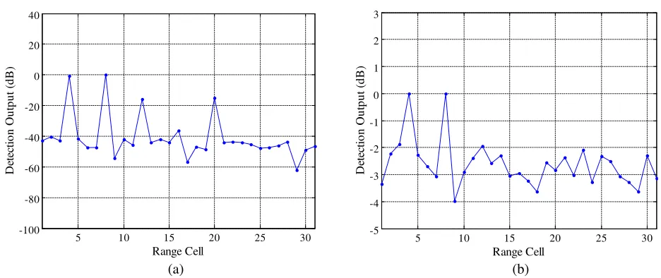
As a contrast, Fig. 6(b) shows the detection output based on GIP nonhomogeneous detector (GIP-NHD). Compared with the proposed method, the limitations of GIP-NHD are mainly embodied in the following two aspects:

1. The test statistics of GIP is η_GIP =X_lHR_LX_l, and R_L is the covariance matrix estimated withL

training samples. So when there are strong target-like signals contained in training samples, deep null will be formed in the direction of the target-like signals. This will lead to signal cancelation phenomenon, severely degrading the detection performance to the weak target-like signals. Exactly as shown in Fig. 6(b), when the training samples contain strong like signals, the weak target-like signals cannot be effectively identified.

2. In addition, conventional GIP-NHD detects and rejects the nonhomogeneous samples directly. However, when the target-like signals are dense, directly excluding the training samples will cause a significant reduction of the sample quantity, which increases the CCM estimation error or, even worse, makes the CCM inversion unrealizable.

5 10 15 20 25 30

-100 -80 -60 -40 -20 0 20 40

Range Cell

D

et

ec

ti

on O

u

tput

(

d

B

)

5 10 15 20 25 30

-5 -4 -3 -2 -1 0 1 2 3

Range Cell

D

et

ec

ti

on O

u

tput

(

d

B

)

(b) (a)

Figure 6. Target-like signal detection. (a) Main beam detection. (b) GIP non-homogeneous detection.

In view of the above questions, we eliminate the target-like signals using the proposed algorithm. After that, we use the joint-domain localized (JDL) STAP [23] to detect the target.

From Fig. 7 we can see that when the training samples contain target-like signals, because of the target self-nulling phenomenon caused by the target-like signals, the target is unable to be identified. In contrast, we reject the nonhomogeneous samples detected by GIP-NHD and use the rest samples to estimate the CCM. As shown in Fig. 7(c), the JDL-STAP based on GIP-NHD fails to detect the target (Because of the rejection of training samples by GIP-NHD, the 4th and 8th range cells have no output). While we apply training samples processed with the elimination algorithm to CCM estimation and STAP weight caculation, the target can be successfully detected. Synthesizing the analysis of Fig. 6 and Fig. 7, we could conclude that the proposed method outperforms traditional GIP-NHD algorithm in scenarios with dense nonhomogeneous samples.

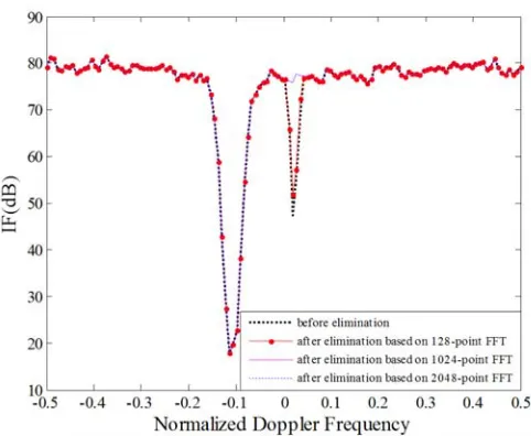
4.2. Improved Factor (IF) Analysis

5 10 15 20 25 30 -40

-30 -20 -10 0 10 20

Range Cell

D

et

ec

ti

on O

u

tput

(d

B

)

5 10 15 20 25 30

-40 -30 -20 -10 0 10 20

Range Cell

D

et

ec

ti

on O

u

tput

(

d

B

)

5 10 15 20 25 30

-40 -30 -20 -10 0 10

Range Cell

D

ete

ctio

n

O

u

tp

u

t (d

B

)

(b) (a)

(c)

Figure 7. Target detection output using JDL. (a) Before eliminating target-like signals. (b) Based on GIP-NHD. (c) After eliminating target-like signals.

1024-point FFT and 2048-point FFT almost coincide and have no null at the Doppler frequencies of the target-like signals. It is seen that both of them can effectively eliminate target-like signals and have similar clutter suppression performance. So we adopt the 1024-point FFT in our algorithm because of its less computational complexity.

4.3. Computational Complexity Analysis

Different from the GIP-NHD directly rejecting the nonhomogeneous samples after detection, the proposed method locates the nonhomogeneous samples and exploits RDSR to eliminate target-like signals, which requires much more computation. And the main computational complexity difference comes from RDSR. So we focus on the analysis of the computation of the RDSR. In order to better illustrate the small computation of the RDSR that we adopted, we compare the improved OMP with traditional RDSR method (i.e., RDSR based on convex optimization) [25, 26]. The total complex multiplications for the RDSR based on convex optimization is O[N_S2N] while the improved OMP is

Figure 8. JDL improvement factor curves.

5. CONCLUSION

This paper proposes a novel nonhomogeneous STAP algorithm for target-like signal elimination based on RDSR. The proposed algorithm utilizes the angle-Doppler spectrum obtained by RDSR to estimate target-like signal and subtract the target-like signal from the training sample. Simulation results illustrate that the proposed algorithm can effectively eliminate the target-like signal and improve target detection performance of the STAP system. In addition, this scheme has low computation complexity, and it is suitable for the practical use.

Based on existing studies, we are currently working on generalizing the present algorithm to more complicated (non-ULA) array structure. We attempt to implement the new algorithm through the rational design of spatial steering dictionary based on array element distribution. Details on such a expansion algorithm are forthcoming.

ACKNOWLEDGMENT

This work was supported in part by the National Natural Science Foundation of China (No. 61771182, No. 61601243, No. 61601167), Aeronautical Science Foundation of China (No. 20162052019), Natural Science Foundation of Jiangsu Province (No. BK20160915).

REFERENCES

1. Brennan, L. E. and I. S. Reed, “Theory of adaptive radar,” IEEE Transactions on Aerospace and Electronic Systems, Vol. 9, No. 2, 237–252, 1973.

2. Melvin, W. L., “A STAP overview,” IEEE Aerospace and Electronic Systems Magazine, Vol. 19, No. 1, 19–35, 2004.

3. Reed, I. S., J. D. Mallet, and L. E. Brennan, “Rapid convergence rate in adaptive arrays,” IEEE Transactions on Aerospace and Electronic Systems, Vol. 10, No. 6, 853–863, 1974.

4. Jeon, H., Y. Chung, W. Chung, et al., “Clutter covariance matrix estimation using weight vectors in knowledge-aided STAP,” Electronics Letters, Vol. 53, No. 8, 560–562, 2017.

6. Ciuonzo, D., A. D. Maio, and D. Orlando, “On the statistical invariance for adaptive radar detection in partially homogeneous disturbance plus structured interference,” IEEE Transactions on Signal Processing, Vol. 65, No. 5, 1222–1234, 2017.

7. Ciuonzo, D., D. Orlando, and L. Pallotta, “On the maximal invariant statistic for adaptive radar detection in partially homogeneous disturbance with persymmetric covariance,”IEEE Signal Processing Letters, Vol. 23, No. 12, 1830–1834, 2016.

8. Rangaswamy, M., P. Chen, J. H. Michels, and B. Himed, “A comparison of two non-homogeneity detection methods for space-time adaptive processing,” Sensor Array and Multichannel Signal Processing Workshop Proceedings, 355–359, Rosslyn, VA, USA, Aug. 2002.

9. Tang, B., J. Tang, and Y. Peng, “Detection of heterogeneous samples based on loaded generalized inner product method,”Digital Signal Process, Vol. 22, No. 4, 605–613, 2012.

10. Shackelford, A. K., K. Gerlach, and S. D. Blunt, “Partially adaptive STAP using the FRACTA algorithm,”IEEE Transactions on Aerospace and Electronic Systems, Vol. 45, No. 1, 58–69, 2009. 11. Rabideau, D. J. and A. Steinhardt, “Improved adaptive clutter cancellation through data-adaptive training,”IEEE Transactions on Aerospace and Electronic Systems, Vol. 35, No. 3, 879–891, 1999. 12. Wu, Y. F., T. Wang, J. X. Wu, and J. Duan, “Training sample selection for space-time adaptive processing in heterogeneous environments,”IEEE Geoscience and Remote Sensing Letters, Vol. 12, No. 4, 691–695, 2015.

13. Wu, Y. F., T. Wang, J. X. Wu, and J. Duan, “Robust training samples selection algorithm based on spectral similarity for space-time adaptive processing in heterogeneous interference environments,”

IET Radar, Sonar &Navigation, Vol. 9, No. 7, 778–782, 2015.

14. Gao, Z. Q. and H. H. Tao, “Robust STAP algorithm based on knowledge-aided SR for airborne radar,”IET Radar, Sonar & Navigation, Vol. 11, No. 2, 321–329, 2017.

15. Sun, K., H. Zhang, G. Li, et al., “A novel STAP algorithm using sparse recovery technique,”

Proceedings of 2009 IEEE International Geoscience and Remote Sensing Symposium, 336–339,

Cape Town, South Africa, Jul. 2009.

16. Herman, M. A. and T. Strohmer, “High-resolution radar via compressed sensing,” IEEE Transactions on Signal Processing, Vol. 57, No. 6, 2275–2284, 2009.

17. Han, S. D., C. F. Fan, and X. T. Huang, “A novel STAP based on spectrum-aided reduced-dimension clutter sparse recovery,” IEEE Geoscience & Remote Sensing Letters, Vol. 14, No. 2, 213–217, 2017.

18. Duan, K.Q., Z.T. Wang, W. C. Xie, et al., “Sparsity-based STAP algorithm with multiple measurement vectors via sparse Bayesian learning strategy for airborne radar,” IET Signal Processing, Vol. 12, No. 5, 544–553, 2017.

19. Yang, Z. C., X. Li, H. Q. Wang, and W. D. Jiang, “On clutter sparsity analysis in space–time adaptive processing airborne radar,”IEEE Geoscience and Remote Sensing Letters, Vol. 10, No. 5, 1214–1218, 2013.

20. Sen, S., “Low-rank matrix decomposition and spatio-temporal sparse recovery for STAP radar,”

IEEE Journal of Selected Topics in Signal Processing Vol. 9, No. 8, 1510–1523, 2015.

21. Ji, C. X., M. W. Shen, C. Liang, et al., “An efficient adaptive clutter compensation algorithm for bistatic airborne radar based on improved OMP application,” Progress In Electromagnetics Research M, Vol. 59, 203–212, 2017.

22. Klemm, R., “Applications of space-time adaptive processing,”IET Digital Library, 2004.

23. Wang, H. and L. J. Cai, “On adaptive spatial-temporal processing for airborne surveillance radar systems,”IEEE Transactions on Aerospace and Electronic Systems, Vol. 30, No. 3, 660–670, 1994. 24. Klemm, R., “Principles of space-time adaptive processing,” The Institution of Engineering and

Technology, London, UK, 2002.

25. Shen, M. W., J. Wang, D. Wu, et al., “An efficient data domain STAP algorithm based on reduced dimension sparse reconstruction,” Acta Electronica Sinica, Vol. 42, No. 11, 2286–2290, 2014. 26. Shen, M. W., J. Yu, D. Wu, et al., “An efficient adaptive angle-doppler compensation approach for