Matrix Method for Antenna Plane Wave Spectrum
Calculation Using Irregularly Distributed Near-Field Data:
Application to Far-Field Assessment
Mohamed Farouq*, Mohammed Serhir, and Dominique Picard
Abstract—The matrix method for the calculation of antenna far-field using irregularly distributed near-field measurement data is presented. The matrix method is based on the determination of the plane wave expansion (PWE) coefficients from the irregular near-field samples using a matrix form that connects the radiated field with the corresponding plane wave spectrum. The plane wave spectrum is used to determine the far-field of the antenna under test (AUT). The matrix method has been implemented, and its potentialities are presented. The validations using analytical radiating model (dipoles array) and experimental measurement (X band standard gain horn antenna) results have demonstrated the efficiency and stability of the proposed method.
1. INTRODUCTION
The characterization of antenna far-field pattern is an important task of antenna measurement
community. Among the existing methods for far-field assessment, we can find direct and indirect
measurement techniques. The direct technique measures the antenna response when illuminated by a plane wave. This is reached directly at the far-field distance or using a compact range. The indirect technique is based on the near-field measurement over canonical surfaces in an anechoic chamber from which the radiation pattern is calculated through near-field to far-field transformation (NFFFT) algorithms. An overview of these algorithms is presented in [1]. The NFFFT are based on an expansion of the electromagnetic field into plane wave (PWE), cylindrical wave (CWE) or spherical wave (SWE). The geometry of the used scanning near-field surface imposes which wave expansion to use [2–7]. The planar near-field measurement technique is used to characterize directive antennas and have enjoyed a great popularity due to the relative simplicity involved in the data acquisition and processing. For the plane wave expansion, Wang [7] has presented a detailed examination of the theory and practice of this technique in 1988.
As an alternative to the wave expansion methods, it is possible to model the AUT through a set of equivalent currents distribution ([8–13]). These currents are set from the near-field measurement data, by solving the inverse radiation problem using the method of moments (MoM) [14]. This is the solution of the integral equations relating the equivalent currents and their radiated field that matches the measured one. From these equivalent currents, it is possible to calculate the AUT radiated field at any point of the space outside the equivalent sources domain. This method needs, however, the AUT a priori information: AUT location, dimensions, type.... The quality of the field reproduced (also the far-field) by the equivalent currents depends on the chosen distribution and spatial positioning of these equivalent electric or magnetic sources.
Newell [15] identified 18 error sources in the antenna planar near field measurements procedure and the impact of each near-field error on the far-field pattern was estimated. In [16], Muth evaluated
Received 9 January 2015, Accepted 30 March 2015, Scheduled 8 May 2015 * Corresponding author: Mohamed Farouq ([email protected]).
the effect of probe displacement errors in the planar near-field measurement procedure on the far-field pattern. In [16] not only the maximum far-far-field errors caused by systematic position errors or the dependence of this maximum on the wave-number were studied, but also it deduced the exact error that contaminated the far-field when the probe displacements were known. Moreover, the theoretical study was carried out with enough generality so that the analysis can be extended to study position errors in cylindrical and spherical scanning geometries. In [17] authors analyzed the same kind of errors but in bi-polar measurements. The NF measured with position errors may be consider either as an erroneous NF or as a NF measured on an irregular meshing. Considering this second situation the position errors may be random but have to be known (laser interferometry is often used for this purpose).
Dealing with irregular measurement data, the near-field plane wave expansion (PWE) based on 2-D Discret Fourier Transform (DFT) allowing the far-field calculation is not possible. Using the fact that the measured field is a band limited function [18], the irregular near-field is interpolated to reconstruct a regular near-field grid, then, the data are processed using classical 2-D DFT algorithm to determine the far-field radiation pattern. This solution based on interpolating the near-field has been presented by many authors and exists in a variety of coordinate systems [19–22]. Wittmann in [23] have proposed an approach to deal with these irregularities by combining unequally spaced DFT [24], interpolation, and the iterative conjugate gradient algorithm. More recently an interesting approach has been presented in [25–27] in which a plane wave expansion is used to calculate near-field to far-field transformation with similar paradigm of equivalent-currents method. This method permits the far-field calculation of the antenna from its near-field sampled over irregular grid. To overcome the computational complexity of this method the Multilevel Fast Multipole Method has been used [28] to perform matrix-vector products and accelerate the resolution of the linear system. The implementation of the fast multipole method proved to be a rather difficult task in part because of its complexity and because of the need to optimize all the steps of this method.
In this paper we present the matrix method to calculate the antenna PWE and consequently the far-field using non-uniformly spaced samples distributed randomly in 3-D rectangular surface (irregularities
inx,yandzdirections), where the Shannon criterion may be broken in limited area of the measurement
surface [18]. The principle of the matrix method proposed here is based on the matrix formulation of the PWE that expresses the linear relationship between the irregularly distributed near-field data and the plane wave spectrum. Solving this linear system, we calculate the plane wave spectrum and the far-field in the half space in front of the AUT.
We aim at introducing the matrix technique for PWE calculation where no interpolation is used and no a priori information are needed to calculate the AUT far-field. The equivalent currents technique, where the a priori information is essential, is popular and we are interested in comparing the two techniques using synthetic and experimental data.
The paper is structured in the following sections. In Section 2 the mathematical developments of the matrix method are presented. Results issued from this method are presented in Section 3 for
different antennas. The first studied AUT is an array of 10×10 infinitesimal dipoles to generate the
irregular near-field data analytically. Then, the far-field results of the proposed method are presented for an X band standard gain horn antenna measured in a planar near-field range at 12 GHz. Finally, a conclusion is outlined in Section 4.
2. THE MATRIX METHOD FOR PLANE WAVE EXPANSION
In this section we present the mathematical basis of the matrix method to calculate the PWE from a rectangular irregular near-field samples distributed randomly in a 3-D domain.
We start by recalling the theory of classical plane wave spectrum for regularly distributed near field data. Then we introduce the matrix method for such case. Finally we extend the matrix method to the
case where the samples are irregularly distributed. Throughout this paper, exp(jωt) time dependence
is suppressed in all the E-field expressions.
The plane wave expansion (PWE) expresses the electric field vector E at the point (xmeas,y,z) of
the measurement surface as a function of the plane wave spectrum vectorF. In our analysis we suppose
that only the tangential components Ey and Ez of the electric field are measured at the plane xmeas
wave spectrumF following
E(xmeas, y, z) = 1 4π2
+∞
−∞
+∞
−∞
F(ky, kz)e−j(kxxmeas+kyy+kzz)dkydkz (1)
F(ky, kz) =
+∞
−∞
+∞
−∞
E(xmeas, y, z)ej(kxxmeas+kyy+kzz)dydz (2)
In practice, the measurement surface can not be infinite andymin≤y≤ymaxandzmin≤z≤zmax.
Accordingly we present the truncated form of (2) as
F(ky, kz) =
ymax
ymin
zmax
zmin
E(xmeas, y, z)ej(kxxmeas+kyy+kzz)
dydz (3)
The near-field is discretized using the sampling steps Δy and Δz over y and z directions.
Fkny, kmz = P p=1 Q q=1
E(xmeas, yp, zq)ej(k n,m
x xmeas+kynyp+kmzzq)Δ
yΔz (4)
E(xmeas, yp, zq) = 1 4π2
N n=1 M m=1
Fkny, kzme−j(kn,mx xmeas+knyyp+kzmzq)Δk
yΔkz (5)
where, kn,mx =
k2−(kn
y)2−(kzm)2, k is the wave-number in free space, Δky = 2π/(ymax−ymin), Δkz = 2π/(zmax−zmin),P = (ymax−ymin)/Δy+1,Q= (zmax−zmin)/Δz+1,N = (kymax−kymin)/Δky+1
and M = (kzmax−kzmin)/Δkz+ 1 with kymin ≤ky ≤kymax and kzmin ≤kz ≤kzmax.
The field and the plane wave spectrum can be expressed as follow: E =Exex+Eyey +Ezez and
F =Fxex+Fyey+Fzez.
Ey(xmeas, yp, zq) = 41
π2 N n=1 M m=1
Fykny, kzme−j(k n,m
x xmeas+knyyp+kmz zq)Δ
kyΔkz (6)
Ez(xmeas, yp, zq) = 1 4π2
N n=1 M m=1
Fzkyn, kmz e−j(kxn,mxmeas+kynyp+kmz zq)Δk
yΔkz (7)
We express the matrix form of (6) and (7) as
Ey(xmeas, yp, zq) =AregularFykyn, kmz Ez(xmeas, yp, zq) =AregularFzkny, kmz
(8)
with
Aregular = ΔkyΔkz 4π2
⎛ ⎜ ⎜ ⎝
e−j(kx1,1xmeas+k1yy1+k1zz1)
. . . e−j(kN,Mx xmeas+kNyy1+kMz z1)
..
. . .. ...
e−j(kx1,1xmeas+k1yyP+k1zzQ) . . . e−j(kN,Mx xmeas+kNyyP+kMz zQ) ⎞ ⎟ ⎟
⎠ (9)
The matrix method consists in the inversion of the equation system (8) where Fy and Fz are the
unknowns.
As an extension, we generalize the matrix method to deal with the irregular distributed data over a known grid, which are due to the errors caused by the probe displacement. In other terms, the irregular grid provides from a slightly modified regular grid. The Near-Field (NF) data are collected over a 3-D grid defined by (xirregmin ≤x
irreg
l ≤xirregmax,yminirreg≤ylirreg≤yirregmax and zminirreg≤zlirreg≤zmaxirreg), for 1≤l≤L,
withL is the number of measured points.
In this situation (irregular distributed data), (8) can be rewritten as follow: ⎧
⎨ ⎩
Eyirreg
xirregl , yirregl , zlirreg
=AirregFykyn, kmz
Ezirreg
xirregl , ylirreg, zlirreg
=AirregFzkyn, kmz
where,
Airreg = ΔkyΔkz 4π2
⎛ ⎜ ⎜ ⎝
e−j(kx1,1xirreg1 +ky1y1irreg+k1zzirreg1 ) . . . e−j(kxN,Mxirreg1 +kNyyirreg1 +kMz zirreg1 )
..
. . .. ...
e−j(kx1,1xirregL +ky1yLirreg+k1zzirregL ) . . . e−j(kxN,MxirregL +kNyyirregL +kMz zirregL )
⎞ ⎟ ⎟
⎠ (11)
Eyirreg = ⎛ ⎜ ⎜ ⎜ ⎝
Eyirreg
xirreg1 , y irreg 1 , z
irreg 1
.. .
Eyirreg
xirregL , yLirreg, zirregL
⎞ ⎟ ⎟ ⎟
⎠, Ezirreg= ⎛ ⎜ ⎜ ⎜ ⎝
Eirregz
xirreg1 , y irreg 1 , z
irreg 1
.. .
Eirregz
xirregL , yirregL , zLirreg ⎞ ⎟ ⎟ ⎟ ⎠ (12)
Fy =
⎛ ⎜ ⎝
Fyky1, k1z .. . FykyN, kMz
⎞ ⎟
⎠, Fz=
⎛ ⎜ ⎝
Fzk1y, kz1 .. . FzkNy , kzM
⎞ ⎟
⎠ (13)
In our problem the near-field measurement is devoted to antenna far-field determination. Indeed,
we take into account only the propagating plane waves (kxn,m =
k2−kn
y
2
−(kmz )2 real) for the
calculation of the plane wave spectrumF. This stay true, since the distance between the probe and the
antenna under test is beyond the evanescent near-field zone. As a consequence, the spatial sampling steps are chosen at a value slightly lower than half a wavelength.
Equation (10) is over determined since the number of equations exceeds the number of unknowns, we look for the least square solution (LSQR) of (10). The LSQR solution passes by the solution of (14).
AHirregEyirreg=AHirregAirregFy
AHirregEzirreg=AHirregAirregFz
(14)
The operator AHirreg is the Hermitian (conjugate) transpose ofAirreg. The least square solutionFy
and Fz of (14) minimize||AHirregE irreg
y −AHirregAirregFy||and ||AHirregE irreg
z −AHirregAirregFz||. In the given example, different direct and iterative methods, the pseudo inverse, conjugate gradient (CG) and LSQR method [29] have been applied. LSQR and CG achieve a small residual of the same order, whereas LSQR shows a slightly faster convergence. The matrix inversion using the pseudo inverse method reveals, as expected, very long computation time, even for rather small matrices. The LSQR method is based on the bidiagonalization procedure of Golub and Kahan [29]. It is analytically equivalent to the standard method of conjugate gradients, but possesses more favorable numerical properties.
Once Fy and Fz are determined, the normal componentFx of the vector spectrumF is calculated
using the property that the region contains no free charges (div(E) = 0))
k·F = 0 kxFx+kyFy+kzFz = 0
Fx=−kyFy+kzFz
kx
(15)
Once the measured near-field plane wave spectrum is calculated the far-field in the spherical
coordinates system (r,θ,φ) is directly determined based on the following expression
Efar-field(r, θ, φ) = jksinθcosφe −jkr
r F (ksinθsinφ, kcosθ) (16)
As it can be seen the mathematical development of the matrix method for the plane wave expansion from irregular near-field data is easy to implement.
3. RESULTS
The matrix method is tested in two situations. In the first situation a numerical radiating antenna
positions are modeled considering the following procedure. First, we create a regular grid in both y
and z directions using respectively the sampling steps Δy and Δz. Then, we add random functions
(Randomy, Randomz defined in Matlab) varying between−1 and +1. These functions allow us to create
an irregular grid in two dimensions. The irregularities are controlled using the weighting factorsχy and
χz. Finally, to generate a three dimensions irregularities we consider a given xmeas to which we add a
random function Randomx varying between 0 and 1 and multiplied by a controlled irregularity factor
χx. This procedure is formulated in (17)
yirregl(p,q)=pΔy+ Randomyχy
zirregl(p,q)=qΔz+ Randomzχz
xirregl(p,q)=xmeas+ Randomxχx
(17)
In the second situation, we measure an X-band standard gain horn antenna in SUPELEC planar near-field range. This measurement setup allows only the near-field measurement over regular grid at certain distance from the AUT. In order to simplify the experimental validation of the matrix method,
we just consider the irregularities created in x direction, because the majority of the existing methods
are not able to take into account this irregularity. This is done by measuring the near field in different
planes x =xmeas. Then, experimental irregular near field data are constructed by choosing randomly
the samples from the different measurement planes for each (yp,zq).
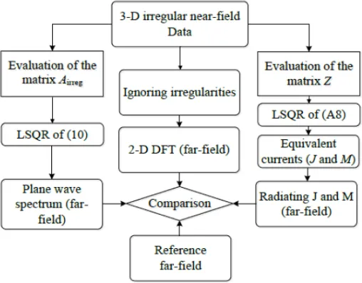
In both situations, the far-field pattern is calculated using the matrix method, equivalent currents method and by DFT while ignoring irregularities and the different obtained far-field patterns are compared with the reference far-field (Fig. 1). In the numerical study the reference far-field is calculated directly. The reference far-field for the experimental study is obtained by DFT of the measured regular
near-field at xmeas = 12 cm.
Figure 1. Validation procedure of the matrix method.
3.1. Numerical Study
The 10×10 z-dipoles array under consideration is composed of equally excited dipoles distributed
regularly over the planeyOz. The dipoles areλ/2 spaced along they andzdirections (λis the working
wavelength). The near-field measurement surface is centered on the axis of the AUT and the field is
collected over a square surface of side 20λ (ymax = −ymin = zmax = −zmin = 10λ). The near field is
of the measurement surface limits the reliable region of the calculated far-field. The reliable far-field
angular region (θvalid and φvalid) is computed as
⎧ ⎪ ⎪ ⎨ ⎪ ⎪ ⎩
θvalid = tan−1
(zmax−zmin)−d 2xmeas
φvalid= tan−1
(ymax−ymin)−d 2xmeas
(18)
where, dis the diameter of the AUT andxmeas is the distance between the AUT and the measurement
plane. In this case of study θvalid = 80◦ and φvalid = 80◦.
In order to evaluate the accuracy of the proposed method, we quantify the deviation between
the co-polar far-field Ecalc issued from the different methods (matrix method and equivalent currents
method) and the co-polar of the exact oneEexact calculated directly from the dipoles radiation pattern,
by means of the root mean square difference of the two far-fields. This quantity is evaluated either on the 2D or 1D far-field pattern. For example, the 2D far-field pattern deviation, i.e., error, is defined as below:
Error(%) = 100
θ,φ|Ecalc (θ, φ)−Eexact(θ, φ)|2 θ,φ|Eexact(θ, φ)|2
, 10◦≤θ≤170◦ and −80◦ ≤φ≤80◦ (19)
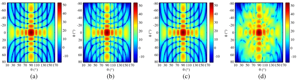
The results are presented and compared with the reference field (Eexact) in Figs. 2(a)–(b)–(c)–(d).
Fig. 2 shows the far-field pattern calculated from a near field measured in irregular positions using
χy,z =χx=λ/10. This means that the irregularity magnitude is λ/5 peak to peak. It is seen that the
use of the matrix method based on the PWE gives a comparable accuracy with the equivalent currents method. Both methods fit very well the actual radiated far-field. In the case where we don’t take into account the irregularities, we use directly the discrete Fourier transform to calculate the plane wave spectrum and the far-field radiation pattern. This is presented in Fig. 2(d). The differences between this far-field and the actual one are important.
10 30 50 70 90 110 130 150 170 -80 -60 -40 -20 0 20 40 60 80 -10 0 10 20 30 40 50
θ ( )o
10 30 50 70 90 110 130 150 170
θ ( )o
10 30 50 70 90 110 130 150 170
θ ( )o
10 30 50 70 90 110 130 150 170
θ ( )o
φ ( ) o -80 -60 -40 -20 0 20 40 60 80 φ ( ) o -80 -60 -40 -20 0 20 40 60 80 φ ( ) o -80 -60 -40 -20 0 20 40 60 80 φ ( ) o -10 0 10 20 30 40 50 -10 0 10 20 30 40 50 -10 0 10 20 30 40 50
(a) (b) (c) (d)
Figure 2. Amplitude of the radiation pattern (co-polar) as a function ofθandφ. (a) Reference pattern, (b) matrix method, (c) equivalent currents method, (d) ignoring irregularities.
The principal plane cuts θ= 90◦ and φ= 0◦ of the co-polar component of the E-field pattern are
presented in Fig. 3 for irregularities associated with χy,z = χx = λ/10. This shows the comparison
between the reference and the far-field pattern obtained using the matrix method, equivalent currents method and when the irregularities are ignored. We note that both methods present a good agreement
with the reference radiation pattern with an error of order 1.1% for θ = 90◦ and 1.6% for φ = 0◦ for
the matrix method. The use of the equivalent currents method leads to errors of 1.6% for θ= 90◦ and
1.4% for φ= 0◦. In the situation where the irregularities are not taken into account, significant errors
in the side lobes of the radiation pattern are induced.
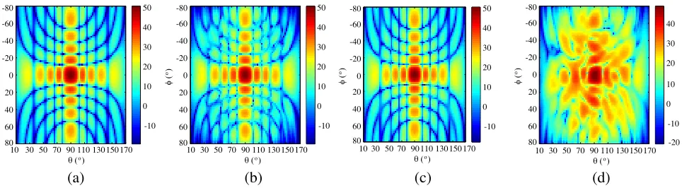
We study the influence of the weighting factorχy,z,χx. Fig. 4 shows the far-field pattern determined
10 30 50 70 90 110 130 150 170 Magnitude (dB) -20 -10 0 10 20 30 40 50 60 Reference Matrix method (PWE) Equivalent currents Ignoring irregularities
Reference Matrix method (PWE) Equivalent currents Ignoring irregularities
θ ( )o
-80 -60 -40 -20 0 20 40 60 80
φ ( )o
Magnitude (dB) -20 -10 0 10 20 30 40 50 60 (a) (b)
Co-polar (φ = 0 )o Co-polar (θ = 90 )o
Error=1.4%
Error=1.6% Error=1.6% Error=1.1%
Error=11.5% Error=10.3%
Figure 3. The far-field (co-polar) comparison at the principal plane cuts. The comparison includes: reference radiation pattern, matrix method, equivalent currents methods and when ignoring irregularities.
10 30 50 70 90 110 130 150 170 -80 -60 -40 -20 0 20 40 60 80 -10 0 10 20 30 40 50
θ ( )o
φ ( )
o
(a) (b) (c) (d)
10 30 50 70 90 110 130 150 170
θ ( )o
10 30 50 70 90 110 130 150 170
θ ( )o 10 30 50 70 90 110 130 150 170
θ ( )o
-80 -60 -40 -20 0 20 40 60 80 φ ( ) o -80 -60 -40 -20 0 20 40 60 80 φ ( ) o -80 -60 -40 -20 0 20 40 60 80 φ ( ) o -10 0 10 20 30 40 50 -10 0 10 20 30 40 50 -10 0 10 20 30 40 -20
Figure 4. Amplitude of the radiation pattern (co-polar) as a function ofθandφ. (a) Reference pattern, (b) matrix method, (c) equivalent currents method, (d) ignoring irregularities.
far-field using the matrix method, the equivalent currents method and when ignoring the irregularities. As it can be seen, increasing the weighting factor influences directly the far-field accuracy especially in the low level far-field areas. Moreover, in the case where we ignore the irregularities the radiation pattern is strongly modified.
In Fig. 5 we present the plane cutsθ= 90◦ andφ= 0◦ forχy,z =χx=λ/5. In these plane cuts the
error between the reference far-field and the far-field pattern obtained using the matrix method is of
order 2.3% for θ= 90◦ and 1.4% for φ= 0◦. The equivalent currents method presents the errors 1.9%
forθ = 90◦ and 1.5% for φ= 0◦ plane cuts. Considering χy,z,x =λ/5 makes the determination of the
far-field pattern in the case where irregularities are not taken into account very critical (green curve).
This leads to high errors in the main and side lobes of order 31.4% forθ= 90◦ and 31.1% forφ= 0◦.
Finally, we are interested in studying the effect of the signal to noise ratio (SNR) over the stability of the matrix and the equivalent currents methods. In fact, this can influence the accuracy of the matrix inversion when calculating the plane wave spectrum or for the equivalent currents determination. To do so, the near-field calculated at irregular positions (xirregl , yirregl , zlirreg) withχ=λ/10 andχ=λ/5 is contaminated with a controlled white Gaussian noise to reduce the SNR.
Figure 6 presents the error values for χ=λ/10 andλ/5 as a function of the near-field data SNR
10 30 50 70 90 110 130 150 170
Magnitude (dB)
-20 -10 0 10 20 30 40 50 60
θ ( )o
-80 -60 -40 -20 0 20 40 60 80
φ ( )o
(a) (b)
Co-polar (φ = 0 )o Co-polar (θ = 90 )o
Magnitude (dB)
-20 -10 0 10 20 30 40 50 60
Reference Matrix method (PWE) Equivalent currents Ignoring irregularities
Error=1.5% Error=1.4%
Error=2.3% Error=1.9%
Error=31.3% Error=31.4%
Reference Matrix method (PWE) Equivalent currents Ignoring irregularities
Figure 5. Principal far-field (co-polar) plane cuts. The comparison includes: reference radiation pattern, matrix method, equivalent currents methods and when ignoring irregularities.
10 20 30 40 50 60 70 80 90 100
0 5 10 15 20 25
(%)
Matrix method (PWE) Equivalent currents
SNR (dB) Error
χ y,z= χ x= λ/10 χ y,z= χ x = λ/5
Figure 6. 2D error values for χy,z =χx =λ/10
and χy,z = χx = λ/5 versus the SNR for the
matrix and the equivalent currents methods.
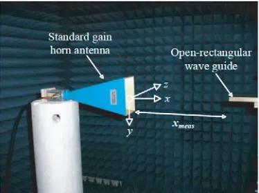
Figure 7. The horn antenna measured in the planar near-field facility.
high values for low SNR near-field data. However, beyond the threshold of 30 dB the error level stays
stable. Moreover, we can see that increasing χ changes slightly the far-field results for both methods
(+3%). These increasing values influence the low level far-field areas.
3.2. Experimental Study
Our purpose is to illustrate the capability of the matrix method for the determination of the far-field of a standard gain pyramidal horn antenna (Fig. 7) measured in SUPELEC planar near-field setup. We
consider the operating frequency of 12 GHz. The horn aperture dimensions are 13 cm×9 cm and the
measurement has been performed using an open-ended rectangular waveguide.
Using the planar translation axes set in the anechoic chamber we measure the tangential components
of the near-field Ey and Ez radiated by the horn antenna over a regular grid (−60 cm≤ymeas ≤60 cm
and −30 cm ≤ zmeas ≤ 30 cm) with Δy = Δz = λ/2.5 sampling criterion in each dimension over
5 different planes (xmeas = 10 cm, 11 cm, 12 cm, 13 cm and 14 cm). Then, the irregular near-field is
constructed by choosing randomly the near-field samples from the 5 measurement grids for each (y,z)
positions.
(a) (b) (c) (d)
-24 -16 -8 0 8 16 24
y/λ
-24 -16 -8 0 8 16 24
y/λ
-24 -16 -8 0 8 16 24
y/λ
-24 -16 -8 0 8 16 24
y/λ
-12 -8 -4 0 4 8 12 z / λ -12 -8 -4 0 4 8 12 z / λ -12 -8 -4 0 4 8 12 z / λ -12 -8 -4 0 4 8 12 z / λ -30 -40 -50 -60 -70 -80 -90 -30 -40 -50 -60 -70 -80 -90 -60 -70 -80 -90 -100 -110 -120 -60 -70 -80 -90 -100 -110 -120
Co-polar Cross-polar Co-polar Cross-polar
Figure 8. Near-field magnitude measured (a), (b) over a regular planar surface and (c), (d) over irregular surface. -60 -50 -40 -30 -20 -10 0 Reference Matrix method (PWE) Equivalent currents Ignoring irregularities -35 -30 -25 -20 -15 -10 -5 Reference Matrix method (PWE) Equivalent currents Ignoring irregularities
30 40 50 60 70 80 90 100110
Magnitude (dB)
θ ( )o
-60 -50 -40 -30 0 20 40 60
φ ( )o
(a) (b)
Co-polar (φ = 0 )o Co-polar (θ = 90 )o
120130140150 -20 -10 10 30 50
0
Magnitude (dB)
Figure 9. Far-field (co-polar) comparison of the principal plane cutsθ= 90◦ andφ= 0◦ in the far-field
validity zone (θvalid ≈60◦ and φvalid ≈60◦). The comparison includes: reference radiation pattern, the
matrix method, the equivalent currents method and when ignoring irregularities.
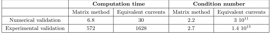
Table 1. Computation time (s) and condition number for matrix method and equivalent currents method.
Computation time Condition number
Matrix method Equivalent currents Matrix method Equivalent currents
Numerical validation 6.8 30 2.2 3 1011
Experimental validation 572 1628 2.7 1.4 1015
co and (b) cross polarization) and for the case of irregularly distributed data ((c) co and (d) cross polarization).
The far-field calculated using the matrix method is compared with the one calculated directly using
DFT of regular near-field data measured at xmeas = 12 cm. This is considered as the reference far-field
pattern. The green curve is associated with irregular near-field data to which a classical near-field to
far field transformation is applied while neglecting the irregularities and by considering xmeas = 12 cm
(medium value). For the equivalent currents assessment (electric and magnetic) we have defined a planar
surface at the horn antenna aperture. The dimensions of this source surface are−9 cm≤ys≤9 cm and
The comparison concerns the principal plane cuts as shown in Fig. 9. The far-field radiation patterns when neglecting irregularities are strongly affected. Using the proposed matrix method and the equivalent currents method the far-field results fits very well the reference one for the co-polarization
plane cutsθ= 90◦ and φ= 0◦.
To get more insight into the efficiency of the proposed matrix method, we have presented in Table 1 the computation times and the condition numbers of the proposed method and the equivalent currents method. As it can be seen the matrix method converges rapidly to the desired solution and presents a low condition number which means that the problem is well posed.
4. CONCLUSION
The matrix method allowing the plane wave expansion of near-field over 3-D irregular grid has been proposed. The technique has shown a good accuracy and high calculation stability. The numerical validation examples have shown that for the near-field data measured at known irregular positions, the far-field can be accurately calculated. Experimental results have been presented using a standard gain horn antenna measured in the SUPELEC planar near-field facility. It has been shown that the radiation pattern of the antenna under test can be reconstructed accurately using the proposed method. However, in the case where we do not take into account the irregularities, the radiation pattern is strongly modified. The matrix method has shown interesting features: a low computational complexity, implementation simplicity, fast convergence to the solution, low condition number and also no a priori information about the AUT is needed in comparison with the well-known equivalent currents method.
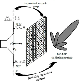
APPENDIX A. THE EQUIVALENT CURRENTS METHOD
According to the equivalence theorem, the field radiated by an antenna can be reproduced from an
equivalent set of electric and magnetic equivalent currents over the virtual surface S placed in the
aperture of the radiating antenna (Fig. A1). The electric field integral equation [30] expresses the AUT
radiated field, in the half space in front of the AUT (x >0), as the superposition of the contribution of
electric (J) and magnetic (M) currents.
Emeas(r) = EJ(r) +EM(r) (A1)
EJ(r) = −jη
4πk Sk
2 J(r)e
−jkR
R +∇
∇
J(r)e
−jkR
R
dS (A2)
EM(r) = −1
4π∇ × S
M(r)e
−jkR
R dS
(A3)
In (A2) and (A3)r(x, y, z) is the position of the observation point and r(x, y, z) is the position
of the source point (equivalent currents). R =|r−r| is the distance between these two points. The
equivalent currents are expressed as M =Myey+Mzez and J=Jyey +Jzez.
The Cartesian components of the electric field can be expressed according to [30] as
EMy(x, y, z) = −
1 4π
y
z
x−xMz1 +RjkR3 e
−jkRdydz (A4)
EJy(x, y, z) = −4jη
πk
y
z
G1Jy +y−yG2y−yJy +z−zJze−jkRdydz (A5)
EMz(x, y, z) = −
1 4π
y
z
x−xMy1 +jkR
R3 e−jkRdydz (A6)
EJz(x, y, z) = −
jη 4πk
y
z
G1Jz+z−zG2y−yJy+z−zJze−jkRdydz (A7)
withG1 = −1−jkRR3+k2R2 andG2 = 3+3jkR−k 2R2
Figure A1. The equivalent currents method for the Far-Field calculation from irregular near-field measured samples.
The numerical representation of the integral equations is a system of linear equations, where the
currentsMy,Mz,Jy andJz are the unknowns. We can write the Equations (A4)–(A7) in a matrix form
Eymeas
Ezmeas
=
Zy,Jy Zy,Jz Zy,My Zy,Mz
Zz,Jy Zz,Jz Zz,My Zz,Mz
⎛⎜ ⎜ ⎝
Jy
Jz
My
Mz
⎞ ⎟ ⎟
⎠ (A8)
where for example:
Zy,Jy =−
jηΔyΔz
4πk e
−jkRG1+y−y2G2 (A9)
where, Δy and Δz are the dimensions of the source rectangular patches. The solution of (A8) is
performed as (10) using LSQR method. As presented in this paper, the mathematical formulation of the equivalent current method seems to be more complicated to handel than the matrix method presented above. Indeed, the accuracy of the equivalent currents method depends on the definition of
the currents surface (S) where these sources are uniformly distributed. This surface is defined based on
the AUT a priori information and the number of considered equivalent sources is of crucial importance. The matrix method is easy and systematic in its application where no a priori information are needed.
REFERENCES
1. Yaghjian, A. D., “An overview of near-field antenna measurements,” IEEE Trans. Antennas
Propagat., Vol. 34, No. 1, 30–45, 1986.
2. Joy, E. B. and D. Paris, “Spatial sampling and filtering in near-field measurements,”IEEE Trans.
Antennas Propagat., Vol. 34, No. 3, 253–261, 1972.
3. Leach, Jr., W. and D. Paris, “Probe compensated near-field measurements on a cylinder,” IEEE
4. Bucci, O. M. and C. Gennarelli, “Use of sampling expansions in near-field-far-field transformation:
The cylindrical case,” IEEE Trans. Antennas Propagat., Vol. 36, No. 6, 830–835, 1988.
5. Wacker, P. F., “Non-planar near-field measurements: Spherical scanning,” NBSIR 75-809, Nat.
Bur. Stand. Boulder, CO, 1975.
6. Hansen, J., Spherical Near-field Antenna Measurements, IEE Electromagnetic Waves Series,
London, 1988.
7. Wang, J. J. H., “An examination of the theory and practices of planar near-field measurement,” IEEE Trans. Antennas Propagat., Vol. 36, No. 6, 746–753, 1988.
8. Petre, P. and T. K. Sarkar, “Planar near-field to far-field transformation using an equivalent
magnetic current approach,”IEEE Trans. Antennas Propagat., Vol. 40, No. 11, 1348–1356, 1992.
9. Sarkar, T. K. and A. Taaghol, “Near-field to near/far-field transformation for arbitrary near-field
geometry utilizing an equivalent electric current and MoM,” IEEE Trans. Antennas Propagat.,
Vol. 47, No. 3, 566–573, 1999.
10. Taaghol, A. and T. K. Sarkar, “Near-field to near/far-field transformation for arbitrary near-field
geometry, utilizing an equivalent magnetic current,” IEEE Trans. Electromagnetic Compatibility,
Vol. 38, No. 3, 536–542, 1996.
11. Las-Heras, F., M. R. Pino, S. Loredo, Y. Alvarez, and T. K. Sarkar, “Evaluating near-field radiation
patterns of commercial antennas,” IEEE Trans. Antennas Propagat., Vol. 54, No. 8, 2198–2207,
2006.
12. Alvarez, Y., F. Las-Heras, and M. R. Pino, “Reconstruction of equivalent currents distribution over
arbitrary three-dimensional surfaces based on integral equation algorithms,”IEEE Trans. Antennas
Propagat., Vol. 55, No. 12, 3460–3468, 2007.
13. Persson, K. and M. Gustafson, “Reconstruction of equivalent currents using a near-field data
transformation with radome application,” Progress In Electromagnetics Research, Vol. 54, 179–
198, 2005.
14. Harrington, R. F., Field Computation by Moment Methods, Oxford University Press, Melboume,
1987.
15. Newell, A. C., “Error analysis techniques for planar near-field measurements,” IEEE Trans.
Antennas Propagat., Vol. 36, No. 6, 754–768, 1988.
16. Muth, L. A., “Displacement errors in antenna near-field measurements and their effect on the far
field,”IEEE Trans. Antennas Propagat., Vol. 36, No. 5, 581–581, 1988.
17. Hojo, H. and Y. Rahmat-Samii, “Error analysis for bi-polar near-field measurement technique,” AP-S Digest Antennas and Propagation Society International Symposium, 1991, Vol. 3, 1442–1445, Jun. 24–28, 1991.
18. Yen, J., “On nonuniform sampling of bandwidth-limited signals,” IRE Trans. Circuit Theory,
Vol. 3, No. 4, 251–257, 1956.
19. Rahmat-Samii, Y. and R. Cheung, “Nonuniform sampling techniques for antenna applications,” IEEE Trans. Antennas Propagat., Vol. 35, No. 3, 268–279, 1987.
20. Dehghanian, V., M. Okhovvat, and M. Hakkak, “A new interpolation method for reconstructing
non-uniformly spaced samples into uniform ones in planar near-field antenna measurements,”IEEE
Antennas and Propagation Society International Symposium, 2003, Vol. 3, 207–210, Jun. 22–27, 2003.
21. Dehghanian, V., M. Okhovvat, and M. Hakkak, “A new interpolation technique for the reconstruction of uniformly spaced samples from non-uniformly spaced ones in plane-rectangular
near-field antenna measurements,” Progress In Electromagnetics Research, Vol. 72, 47–59, 2007.
22. Bucci, O. M., C. Gennarelli, and C. Savarese, “Interpolation of electromagnetic radiated fields over
a plane by nonuniform samples,” IEEE Trans. Antennas Propagat., Vol. 41, No. 11, 1501–1508,
1993.
23. Wittmann, R. C., B. K. Alpert, and M. H. Francis, “Near-field antenna measurements using
nonideal measurement locations,”IEEE Trans. Antennas Propagat., Vol. 46, No. 5, 716–722, 1998.
25. Schmidt, C. H., M. M. Leibfritz, and T. F. Eibert, “Fully probe-corrected near-field far-field
transformation employing plane wave expansion and diagonal translation operators,”IEEE Trans.
Antennas Propagat., Vol. 56, No. 3, 737–746, 2008.
26. Schmidt, C. H. and T. F. Eibert, “Assessment of irregular sampling near-field far-field
transformation employing plane-wave field representation,” IEEE Magazine Antennas Propagat.,
Vol. 53, No. 3, 213–219, 2011.
27. Qureshi, M. A., C. H. Schmidt, and T. F. Eibert, “Adaptive sampling in multilevel plane wave based
near-field far-field transformed planar near-field measurements,” Progress In Electromagnetics
Research, Vol. 126, 481–497, 2012.
28. Schmidt, C. H. and T. F. Eibert, “Multilevel plane wave based near-field far-field transformation
for electrically large antennas in free-space or above material halfspace,” IEEE Trans. Antennas
Propagat., Vol. 57, No. 5, 1382–1390, 2009.
29. Paige, C. C. and M. A. Saunders, “LSQR: An algorithm for sparse linear equations and sparse
least squares,” ACM Trans. Mathematical Software, Vol. 8, No. 1, 1982.