Improving Deep Learning Image Recognition Performance Using Region of Interest Localization Networks

(1)

Scholarship@Western

Electronic Thesis and Dissertation Repository

4-10-2017 12:00 AM

Improving Deep Learning Image Recognition Performance Using

Region of Interest Localization Networks

AbdulWahab Kabani

The University of Western Ontario

Supervisor

Mahmoud R. El-Sakka

The University of Western Ontario Graduate Program in Computer Science

A thesis submitted in partial fulfillment of the requirements for the degree in Doctor of Philosophy

Follow this and additional works at: https://ir.lib.uwo.ca/etd

Part of the Artificial Intelligence and Robotics Commons

Recommended Citation Recommended Citation

Kabani, AbdulWahab, "Improving Deep Learning Image Recognition Performance Using Region of Interest Localization Networks" (2017). Electronic Thesis and Dissertation Repository. 4485.

https://ir.lib.uwo.ca/etd/4485

This Dissertation/Thesis is brought to you for free and open access by Scholarship@Western. It has been accepted for inclusion in Electronic Thesis and Dissertation Repository by an authorized administrator of

(2)

Abstract

Deep Learning has been gaining momentum and achieving the state-of-the-art results on many visual recognition problems. The roots of this field can be traced back to the 1940s of the 20th century. The field has recently started delivering some interesting results on many image understanding problems. This is mainly due to the availability of powerful hardware that can accelerate the training process. In addition, the growth of the Internet and imaging devices such as mobile phones and cameras has contributed to the increase in the amount of data that can be used to train neural networks. All of these factors have contributed to the success of deep learning on large scale image understanding tasks.

Many image understanding problems do not have large training data. This is especially true in many special purpose datasets such as medical images, astronomical images, and environ-mental images. These application do not have large training datasets because unlike natural images, users do not typically take these images and upload them to the web. In addition, some of these applications, such as medical imaging, have many restrictions on sharing the data in order to protect the privacy of the patients. Finally, the labeling process needed for training natural images can be done by any person, unlike special purpose datasets. For example, in medical imaging, the images must be labeled by medical or clinical experts in the field. This results in datasets that are normally much smaller than natural images datasets as these experts have limited time to invest in the creation of the training sets.

Luckily, in many of these applications, the most discriminative features may be present in a small region of interest. In this work, we present a method of training deep learning models on problems with low number of training images. We will do that by localizing a region of interest in these images, which will help reduce the problem of overfitting. In this thesis, two localization architectures are introduced, namely: the standard localization network and the wide localization network (wide net). The latter has several advantages which we explain thoroughly.

(3)

heads. We will study how localizing the region of interest can be used to make deep learning work on such a small dataset.

The second problem we will study is the estimation of the ejection fraction and left ventri-cle volume by analyzing cardiac MRI images. Automatically estimating the ejection fraction and volume of the heart can help in identifying and diagnosing several cardiac health issues. Similarly, this dataset contains only a small number of training subjects.

Keywords: Localization, Detection, Recognition, Artificial Neural Networks, Deep

Learn-ing, Convolutional Neural Network, Image Classification, Whale Localization, Whale Detec-tion, Whale RecogniDetec-tion, Cardiac MRI, Left Ventricle, Automatic Ejection Fraction Estimation

(4)

Co-Authorship Statement

During my PhD studies, I was the main author in 8 papers. This thesis is a summary of 4 pa-pers out of those 8 papa-pers. Appendix A contains a list of the papa-pers that were published during my PhD. A copyright release information about the papers included in this thesis is available in Appendix B . I am the primary author in all of the papers that were published during my doctoral studies. In all of these papers, Dr. Mahmoud El-Sakka was the co-author.

(5)

I would like to thank Dr. Mahmoud El-Sakka for giving me the chance to do my graduate work under his supervision. His support made this work possible.

My family (father, mother, brother) were the source of my strength during the most difficult times during my studies. We have not seen each other for the past 6 years, I hope we meet again soon.

(6)

List of Appendices

Appendix A: List of Papers Published During My Doctoral Studies . . . 82 Appendix B: Copyright Release . . . 84

(13)

Shortcut Description

CNN Convolutional Neural Network Convnet Convolutional Neural Network

CPU Central processing unit D Diastolic Volume EF Ejection Fraction

FCN Fully Convolutional Neural Network GPU Graphics processing unit

IoU Intersection over Union LTSM Long Short Term Memory Networks

MAE Mean Absolute Error

Standard Net The Standard localization neural network RAM Random Access Memory

ReLU Rectified Linear Units ResNet Residual Network

RMSE Root Mean Squared Error ROI Region of Interest

S Systolic Volume

VGG Visual Geometry Group Neural Network Wide Net The Wide Localization Neural Network

(14)

Chapter 1 Introduction

1.1 The Deep Learning Journey

Researchers have always wanted to create machines that can perform intuitive tasks such as: understanding images, speaking, and interacting with humans. Ironically, even though these tasks are performed by humans with no effort, explaining how these tasks can be performed is not straightforward. Because of this, it is difficult for computers to perform these tasks. Indeed, computers are good at things that can be easily described by writing a piece of code. Generally speaking, there have been two approaches to creating machines that can perform

intelligent tasks, namely: the rule based approach and the experience based approach. The

rule based approach involves having humans specify a set of rules that describe the solution to the problem. On the other hand, the experience based approaches involves feeding data into the machine and having the computer learn from the experience over time. Over the past few years, the latter approach has been showing some positive results. Deep Learning[24] is a field in machine learning which involves stacking a set of layers together in order to learn to accomplish a task. The deep learning model can learn complex knowledge because of its hierarchical nature.

(15)

the data (the images). These features are then passed to the model so that the model can learn to classify the image. This greatly reduces the number of parameters that need to be learned. In addition, the input to the model is a feature vector that contains a set of high level features that the human views as important. The success or failure of the learning process relies heavily on how good the features are. This has lead to the development of a lot of techniques and practices to perform feature engineeringon the raw input data. Feature engineering and in-formation representationare essential when dealing with many types of classifiers including logistic regression, SVM, etc. The Deep learning approach is however different. Normally, deep learning involves feeding raw data into the model and the model will learn low level rep-resentation of the data (in the bottom layers), medium level reprep-resentation in the intermediate layers, and high level abstract representation at the top layers.

Deep learning is more suitable for problems where it is difficult to know what kind of fea-tures that should be extracted from the data.Representation learning[24] involves the process of learning not only the output of the problem but also the appropriate set of representations for the problem (the set of features that should be used to describe the problem). Indeed, these features may be really good that they can be used to solve other similar problems. For instance, a model trained to perform image classification can also be used to perform semantic segmen-tation [56]. In the visual recognition problem, deep learning performs really well because it is very difficult to extract reliable features from images. Factors such as image brightness and background occlusion can change the way objects appear in different images.

(16)

1.1. TheDeepLearningJourney 3

this has not be shown to be true as of the time of writing this thesis. Some architectures are more suitable for certain tasks than others. For example, convolutional neural networks[51] are a special type of neural networks that are suitable for visual recognition problems. These networks involve having layers with limited connectivity to simulate a behavior similar to con-volution. These types of networks date back to the 1980s [19]. On the other hand,long short term memory networks(LTSM) [34] are more suitable for natural language processing tasks.

As mentioned earlier, deep learning is not a new field. However, it only started delivering good results recently. There are two main reasons for the resurrection of the field. First, the introduction of powerful hardware that can be used to speed up the training process of the deep learning models. Graphical Processing Units (GPUs) are mainly used to accelerate the output to a computer display. However, over the past few years, they are being used in image processing, computer graphics, and deep learning. This is largely due to their parallel structure which is more suitable than the CPU when working on these types of applications. With respect to deep learning, these devices can train models with around 80x speed up compared to the general purpose CPU.

Second, the availability of large amounts of labeled training data made training deep learn-ing models possible. This data (images, videos, sounds, etc...) are largely generated by users and hosted on the web. In other words, the availability of cameras, mobile phones, and com-puters contributed to the increase in the amount of training data available to train deep learning models. It is important to note that typically deep learning models require a lot of training data in order to achieve the desired results. Not providing enough training data can lead to overfitting. Overfitting happens when the model performs really well on the training data but fails to generalize well to unseen data. The introduction of large training data sets helped in boosting the performance of deep learning models. Some of these data sets include PASCAL VOC [16, 15], ADE20K [92] and the Imagenet challenge [11, 73].

(17)

step, an input is passed through the network until it hits the output layer. Then an error value based on a predefined loss function is calculated and used to calculate the error of each neuron in the network. Finally, the error values associated with each neuron are used to compute the gradient of the loss function with respect to the current network weights. In the second step, the weights are updated based on the gradient that was computed.

Deep learning has been very successful over the past few years in supervised learning. The main difference between supervised and unsupervised training is that in the supervised setting, the desired output value is provided along with the training data. For instance, if we want to train a deep learning model to detect whether an image shows a malignant or benign tumour, we need to provide some images as training data. In a supervised setting, we also have to provide labels to describe the type of tumours in each of the training images. Most of the success that deep learning showed over the past few years was based on supervised learning. However, unsupervised learning has been a very active area of research [50, 66, 25, 27, 63].

(18)

1.1. TheDeepLearningJourney 5

images datasets such as Imagenet [11, 73] that includes millions of images.

There are many datasets with very small number of images. The galaxy zoo challenge [12, 85, 1] involves training models to classify the morphology of the galaxies. These images were acquired using a telescope and include around 60,000 images. The Diabetic Retinopathy [42] contains around 35,126 training images (around 17,563 per subject). The Right whale recognition dataset [43] that we will study contains only 4,544 training images. Finally, the left ventricle volume estimation dataset [41] that we will study has only training data for 500 subjects.

One way to bring the power of deep learning to smaller datasets is to perform transfer learning [32, 87, 64, 89]. However, there are several issues with this. First, pre-training a deep learning model on a large dataset such as the Imagenet [11, 73] may not be very effective on some special types of problems such as medical imaging. This is because the medical images are very different from the natural images. The second problem is a legal issue. Pre-training a model on Imagenet [11, 73] may be problematic because this dataset can only be used for research purpose.

CNNs have achieved the state-of-the-art results on many classification problems [48, 79, 31, 54, 75]. For instance, ResNet[31] is an architecture that can be trained with very large number of layers while being resilient to the vanishing gradient problem [3]. There has been an interest in translating this success into other tasks such as detection [67, 22, 68, 21] and

semantic segmentation[56, 62, 17, 88, 29, 7, 90].

(19)

models for semantic segmentation [56, 62, 17, 88, 29, 7, 90] rely on pre-trained classification models because the amount of training data available in classification problems far exceeds the amount of training data for semantic segmentation even though the latter is more challenging. This is because labeling images for segmentation tasks is very time consuming. The simplest way to make a classification model work for semantic segmentation involves dropping the dense layers and replacing them with 2D convolutional layers.

Most of the current semantic segmentation models are based on Fully Convolutional Neural Networks (FCN) [56]. In [86], a detailed study about the use of ResNet [31] in semantic segmentation was conducted. An attention mechanism that can learn to weight the multi-scale features at each pixel location was proposed in [8]. Typically, in these types of models, they accept a multi-scale input (an image resized to different scales). They perform really well on objects at small scales. PSPNet [90] showed that using global and local clues about the image can boost the performance on the image segmentation challenge.

It may be useful to increase the size of the receptive field. Dilated convolution[88, 7] can be used to achieve this. The inspiration came from a signal processing algorithm for wavelet decomposition called algorithme a trous [35]. In [88], it was shown thatDilated convolution

has nice properties that makes it ideal for dense prediction in semantic segmentation. The main advantage of using dilated convolution is that it can be used to aggregate multi-scale informa-tion while maintaining a low number of parameters. The architecture is composed of 8 layers with different dilation rates. This architecture can be embedded into another base architecture that was trained on the imagenet challenge [11, 73]. Some semantic segmentation models [28] rely on the intermediate layers because they tend to carry a relatively high resolution infor-mation in addition to the abstract inforinfor-mation that can be used to perform the classification. RefineNet [53] was proposed as a multi-path network in order to exploit features at different levels. Finally, the semantic segmentation performance of any model can be improved using conditional random fields (post-processing operation) as shown [91].

(20)

1.2. Region ofInterestLocalization 7

[62, 13, 7], deconvolution was used to upsample the feature maps from the top layer in order to increase their resolution. The other way is to use dilated convolution [88] which is similar to convolution with holes in between. This allows for capturing multi-scale features without downsampling and in a relatively efficient way.

1.2 Region of Interest Localization

While the methods mentioned previously achieve excellent results on semantic segmentation, all of them rely on pre-trained data to achieve the required results. As a consequence, they have a large GPU RAM requirement because they depend on adding layers to models that were trained on classification tasks. We are interested in developing region of interest (ROI) model that have lower memory requirement. These models will be used as a means of pre-processing the data to simplify the classification problem (in this thesis: the whale recognition problem (Chapters 2 and 3) and the left ventricle volume estimation problem (Chapters 4 and 5)). Therefore, these models need to deliver the results as fast as possible and with low memory consumption. In other words, detecting the region of interest is a sub-task that can simplify the main problem (Right whale recognition or left ventricle estimation) and we are interested in an efficient solution that can perform this task.

(21)

wanted to achieve is being able to perform region of interest localization with different shapes whether the region of interest is a point, circle, triangle, rectangle, or irregularly shaped region of interest.

We introduce two architectures that can be used for localizing regions of interest (ROI) in an image. The two architectures are: the standard network (standard net) and the wide localization network (wide net). Some of the factors that influenced the design of these networks are the following:

• Because the networks will be used as a pre-processing step, they should be trained in a relatively short period of time.

• The networks should work well on machines with relatively low computing power.

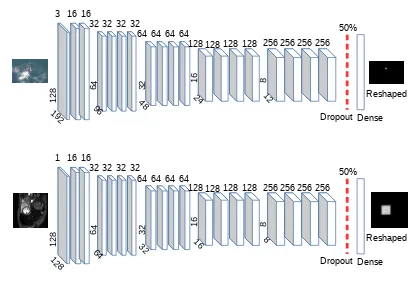
• The networks should be able to learn an ROI of arbitrary shape (not just rectangle ROI). Figure 1.1 shows the architecture of the standard net applied on two separate problems that we will cover in this work. In the first row, the network was trained to localize the bonnet (a point located on the head of the whale). The second row shows how the network can be used to predict the location of the left ventricle. As shown in the two problems, the network can have different input sizes depending on the problem.

Let’s take the first row in Figure 1.1 as an example. The input of the architecture is an image of size 128×192. The ground truth is a flattened mask of size 128 ×192 = 24,576 pixels. In other words, the output of the network is a layer with 24,576 possible classes. The output layer is simply a flattened mask and reshaping this layer gives us back the predicted mask. The pixels with the highest intensities represent the location of the interest point.

(22)

1.2. Region ofInterestLocalization 9 12 8 64 64 32 32 16 16 8 8

1 16 16

32 32 32 32

64 64 64 64

128 128 128 128 256 256 256 256 50% Dropout Dense Reshaped 12₈ 12 8 192 64 96 32 48 24 16 12 8

3 16 16

32 32 32 32

64 64 64 64

128 128 128 128 256 256 256 256 50%

Dropout Dense Reshaped

Figure 1.1: The standard net architecture: this figure shows the architecture of the standard localization net. In the first row, a input image is passed to the network and the bonnet (a point located on the head of the whale) can be localized after training the network. In the second row, the network predicts the location of the left ventricle from a cardiac MRI image. The network can have different input sizes depending on the problem.

Because the last layer in the network is softmax, pixels in the predicted mask are probabil-ities that range between 0 and 1 and that sum up to 1. It is very important to ensure that the ground truth (the labels) follow the same rules. In order to do that, we rescale the true mask (or the true labels) by dividing each pixel by the sum of the mask as shown in the Equation 1.1:

yi j =

pixeli j

PH

i=1

PW

j=1pixeli j

(1.1) where pixeli j is the pixel value at row i and column j. yi j is the normalized pixel value such

thatyi j ∈[0,1] andP H i=1

PW

j=1yi j =1.

(23)

Equation 1.1, the network will not converge.

There are several limitations to the standard localization network. Here are some of them:

• Because the last layer is dense (fully connected), the number of parameters can grow very quickly.

• The network cannot be trained to learn more than one ROI. For instance, when applying this network to the whale recognition problem. We had to train two networks: one is used to localize the bonnet and the other is used to localize the blow hole.

• The network cannot learn to segment an arbitrary shaped ROI. This is because while the top layers has highly abstract information, the spatial resolution is lost due to the pooling layers.

• The output mask requires thresholding in order to produce a binary mask. The results may vary depending on the thresholding model.

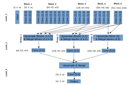
The wide localization network (wide net) is a better alternative to the standard localization network. The architecture of this model is shown in Figure 1.2. This network is capable of performing segmentation and producing region of interests at a very low processing power. The network is composed of three levels: Level 1 is simply a set of convolutional and pooling layers. Level 2 involves merging the last layer from each block in level 1 in three different ways. Three types of merging is done: type 1 involves merging (block 2, block 3, block 4, block 5), type 2 involves merging (block 3, block 4, block 5), and finally type 3 involves merging (block 4, and block 5). Type 1 carries a combination of high resolution features along with highly abstract features. On the other hand, Type 3 carries only abstract features. Finally, in level 3, the outputs of level 2 are combined and a mask is produced.

(24)

1.2. Region ofInterestLocalization 11

(3, h, w)

C on v (5 ,5 ) C on v (5 ,5 ) C on v (3 ,3 ) C on v (3,3 ) C on v (3 ,3 ) C on v (3 ,3 ) C on v (3 ,3 ) C on v (3 ,3 ) C on v (3 ,3 ) C on v (3 ,3 ) C on v (3 ,3 ) C on v (3 ,3 ) C on v (3 ,3 ) C on v (3 ,3 ) C on v (3,3 ) C on v (3 ,3 ) C on v (3 ,3 ) C on v (3 ,3 ) C on v (3 ,3 ) C on v (3 ,3 ) In pu t

(32, h, w) (64, h/2, w/2) (128, h/4, h/4) (256, h/8, h/8) (512, h/16, h/16)

Block_1 Block_2 Block_3 Block_4 Block_5

Upsample Blocks (3,4,5) & Merge blocks (2,3,4,5)

(128, h/4, w/4) (64, h/2, w/2)

Upsample Blocks (4,5)

& Merge blocks (3,4,5) & Merge blocks (4,5)Upsample Block (5)

Conv (5,5)

Conv (5,5) Conv (5,5)

Upsample & Merge

(256, h/8, w/8)

Conv (5,5) Output

(32, h, w)

(oc, h, w)

L ev el _1 L evel _2 L evel _3 G ro u p _1 G ro u p _2 G rou p _3

Figure 1.2: The architecture of wide net: the network is composed of three levels. Level 1 is just like any typical recognition network. Level 2 involves merging the last layer from each block in level 1 in three different ways. Finally, in level 3, the outputs of level 2 are combined and a mask is produced. Abbreviations: h is the height of the image, w is the width of the image, oc is the output channel size.

features, we use Max-pooling in level 1. As a result, the layers in each block in level 1 will have different sizes. In order to combine them together in level 2, we use upsampling to en-suring that the layers can be merged. This network has a low processing footprint and was previously tested on a device with only 3.5 GPU memory.

(25)

50 50 100 100

150 150 200 200

50 100

150 200 W_layer(n)

Hla

ye

r(

n

)

2 × W_layer(n)

2

×

H la

ye

r(

n

)

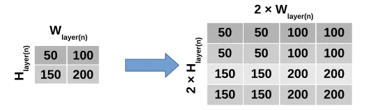
Figure 1.3: The units in a layer can be upsampled by repetition. The unit is repeated across two dimensions to upsample the layer. This is a non-parameterized operation that does not require parameters optimization during training. In order to reproduce a high resolution region of interest, the upsampled layer is combined with layer(s) with higher resolution.

resolution.

There are several advantages to this architecture over the standard architecture:

• It is a very efficient architecture with lower number of parameters.

• The network may have several output channels. This means that it can be trained to localize several ROIs simultaneously.

• The network can learn to identify an arbitrary shapped ROI including segmentation.

• The output mask can be thresholded simply by using the threshold value of 50%. This is because the last layer has a sigmoid activation.

1.3 Right whale Recognition

(26)

1.3. Right whaleRecognition 13

kind, it is very difficult to train a deep neural network with such a small data set. The highest accuracy we were able to achieve on this dataset when training on the images directly (without localization) is 8%. In order to improve the results and overcome this limitation, we can train models to localize the head of the whales. After that, we can train models to recognize the whales. This greatly reduces the amount of viewpoint variance making it possible to train a classification model to recognize the whale.

The main reason for why the dataset is small is because Right whales are endangered species. In addition, labeling these images require a marine biologist who is expert in these animals to perform this task. Unlike general and natural images, labeling these types of images is expensive because a random person cannot be used to label the data.

Historically, Right whales were the subject to harsh hunting since the 17th_{century. Some}

researchers believe that the name ‘Right whale’ comes from the fact that this is the ‘right’ type of whale for hunting. These whales were considered to be ideal for hunting for many reasons such as their tendency to live close to the shore, being rich in whale oil, and the fact that their bodies float when killed. Despite becoming protected species since 1949, the population is still endangered with being entangled in fishing gear, and collision with ships accounting for around 50% of deaths.

Right whales can be recognized by studying the callosities pattern on their heads. Manually classifying whales is a very time consuming process and automating this process can help scientists focus on their conservation efforts. Each Right whale has a unique callosities pattern on its head. These callosities pattern can be used to identify Right whales just like fingerprint pattern can be used to identify humans. We developed a model that can automatically recognize individual whales by analyzing the callosities pattern on their heads. The solution we describe in Chapter 2 was ranked 5th_{(out of 364 teams) in a Kaggle challenge [43] to solve this problem.}

This solution was based on the standard localization network. In Chapter 3, we improve the solution by using the wide net.

(27)

set is very small while the number of classes (individual whales) is large. Indeed, the number of individual whales (the classes we want to predict) is 447. Second, there is a huge variation in the clarity of each image. Finally, the size of each image is very large making it very difficult to load these images into the GPU.

Since the head of the whale occupies only a small area in the whole image, localizing the region of interest is very important. Localizing the region of interest can help the classification model focus on the most discriminative features and avoid irrelevant features such as features in the surrounding water. Normally, a deep learning classification model can learn to ignore irrelevant features by training it on large datasets. However, because this dataset [45] is very small with many classes including only one image, it is important to train the classification model only on the important features.

Here is a summary of the solutions that achieved the best results on this dataset. Deep learning have been very successful in recent years with visual recognition problems. However, it was very difficult to make it work for this type of data. This is mainly because the size of the data is very small. Anil Thomas from Nervana Systems [82] suggested locating the bonnet and the blow hole on the whale. The solution which is based on a deep learning library called Neon [78] used these two points to extract a patch that contains the whale’s head. This approach proved to be very effective. First, it made the training process much faster because the training is being done on smaller images. Second, these head patches are better than the original images for training a deep learning model. This is mainly because training on these head patches made the model focus only on the most discriminative features (the head callosities) and ignore unimportant features such as features from the surrounding water.

(28)

1.4. LeftVentricle andEjectionFractionEstimation 15

introduced [81]. This team used a classifier that is an ensemble of deep neural networks with different variations of the VGG-Net [75] and ResNet [31].

The DeepSense.io team [5] that was ranked in the first position also used a multi-stage approach. This team produced a solution [5] that involves localizing the head of the whale and aligning it afterwards. They report that aligning the head of the whale is very important to achieve good results. Their final solution is based on combining the predictions of different deep learning models.

1.4 Left Ventricle and Ejection Fraction Estimation

The second problem we will discuss in chapters 4 are 5 is the problem of left ventricle volume and ejection fraction estimation. Cardiologists can assess cardiac function by analyzing the end-systolic and end-diastolic volumes, and ejection fraction. These values can be manually measured by a cardiologist but the process is slow and time consuming. We introduce an automated method that can estimate these values. We developed our method on a data set with 500 training studies, 200 validation studies, and tested it on 440 testing studies. The data set is compiled by the National Institutes of Health and Children’s National Medical Center [41].

In general, left ventricle volume can be estimated by detecting it and segmenting its cavity [55, 57, 20, 44]. Once the cavity (the blood pool) is segmented, the volume can be calculated by summing up the sub-volumes of all slices according to simpson’s rule.

In Chapter 4, we take a slightly different approach and estimate the volume using a convo-lutional neural network. In Chapter 4, we were able to estimate the volume with around +/ -15 ml mean absolute error. Furthermore, we were able to estimate the ejection fraction with

(29)

estimated.

(30)

Chapter 2 Right whale Recognition using the

Standard Localization Network

2.1 Introduction

The North Atlantic Right whales [45] is an endangered species with around 450 whales left. Historically, Right whales were the subject to harsh hunting since the 17th _{century. Some}

researchers believe that the name ‘Right whale’ comes from the fact that this is the ‘right’ type of whale for hunting. These whales were considered to be ideal for hunting for many reasons such as their tendency to live close to the shore, being rich in whale oil, and the fact that their bodies float when killed. Despite becoming protected species since 1949, the population is still endangered with being entangled in fishing gear, and collision with ships accounting for around 50% of deaths.

Right whales can be recognized by studying the callosities pattern on their heads. Manually classifying whales is a very time consuming process and automating this process can help sci-entists focus on their conservation efforts. We used a unique data set provided by the National

0_{The majority of this chapter was originally published in: AbdulWahab Kabani, and Mahmoud R. El-Sakka}

“North American Right whale Recognition using Very deep and Leaky Neural Network”, Journal of Mathematics Applications, Vol 5., 2016. [38]

(31)

Oceanic and Atmospheric Administration [45],[43] to develop a model that can automatically recognize individual whales by analyzing the callosities pattern on their heads. The solution we describe in this paper was ranked 5th(out of 364 teams) in a Kaggle challenge [43] to solve this problem.

When working on this problem, we faced several challenges. First, the size of the training set is very small while the number of classes (individual whales) is large. Second, there is a huge variation in the clarity of each image. Finally, the size of each image is very large making it very difficult to load these images into the GPU.

To overcome these challenges, we first localize and normalize the body with respect to rotation. After that, we localize the head of the whale. Finally, the whale is recognized using the callosities pattern on its head. These steps reduce the image size and ensure that we can fit the data into the GPU.

In this chapter, we will present general overview. Information about the data that we used will be presented in Section 2.2. Sections 2.3 and 2.4 describe the methods we used to localize the body and head of the whale, respectively. In Section 2.5, we present the model that we used to recognize the whales. The results are introduced in Section 2.6. Finally, we conclude our work in Section 2.7.

2.2 Method Overview

An overview of our method is presented in Figure 2.1. While the main task is to recognize the individual whales IDs, we could not do that directly on the original images. This is because the original images are huge and trying to fit them in the GPU during recognition is not feasible.

(32)

2.3. BodyLocalization 19

1% 90% ... 2%

Bonnet and Blow Hole Masks Input

Image Train two masks localizer

Localize & Rotate Body

Train a model to localize the head Head

Mask Localize the Head Train a model to recognize whales

Whale IDs Probability Distribution

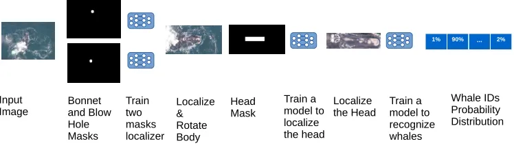
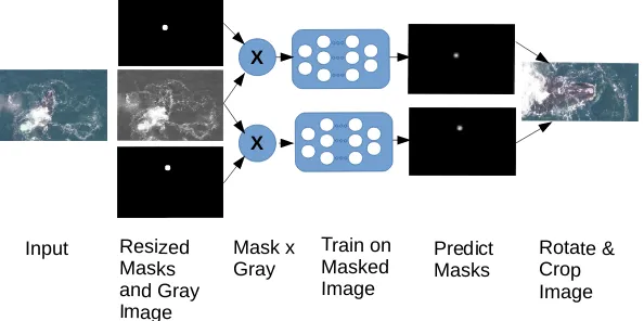
Figure 2.1: The overview of the method: First, two models are trained to localize the bonnet and the blow hole, respectively. Then, using these points, the body of the whale is localized and rotated so that the body has angle=0 with the x axis and the head is pointing east. After that, a model is trained to localize the head of the whale. Finally, a model is trained to produce a probability distribution over all possible whales.

model is trained to produce a probability distribution over all possible whales.

2.3 Body Localization

In this section, we describe how we trained a model to localize the body of the whale and normalize it with respect to rotation. The trained model will be able to take the original image as input and produce an output where the image is cropped and the whale is facing east. This is very important in order to train the classification model (presented in Section 2.5). Figure 2.2 shows a random sample of the input images that we pass to the model in order to localize the whale body.

This is a very important step for many reasons. First, localizing the body and the head (in Section 2.4) helps the model focus on the important features on the whale body rather than on features in the surrounding water. Because there are many classes with very few training images, focusing on the important features in the image (the callosities on the top of the head) is essential to alleviate overfitting.

(33)

A B C

1

2

3

4

Figure 2.2: A random sample of images: These images were captured during several aerial surveys and under different lighting and environmental conditions (note images A1, B2, B4, C4). In addition to these variations, there are many others obstacles, which make these images very challenging. For instance, for many whales the head is not clear because the whale is blowing water as in images C1 and C3. Some images contain more than two whales like in images C2 and B3. In images A2 , C3, and B4, the foreground/background contrast is very low. Water reflection can make recognition very difficult like in image C4. The size of the whale with respect to the background (like the on in image B2) is another challenge.

a lot surrounding water. For example, Figure 2.3 shows two head crops, one crop is for a whale that has 0 degrees angle with the xaxis and another one with around 135 degrees angle. It is clear that the one in the latter crop contains far more water.

(34)

Figure 2.3: Comparison between two head crops. The one on the left is taken from an image where the angle of the body of the whale with the xaxis is 135 degrees. On the other hand, the one on the right is the result of normalizing the angle of the body so that it is 0 degrees. The figure also shows the locations of the bonnet and the blow hole. Two localizations models are trained to recognize the bonnet and the blow hole, respectively. Then, using these two points, we can calculate the angle with thexaxis and rotate the whale accordingly.

used to train two convolutional autoencoders. After that, the head was extracted and rotated. We use a similar approach. However, rather than training a convolutional autoencoder, we trained a deep neural network with the units in the output layer corresponding to individual pixels in the masked image. Figure 2.4 shows a summary of the body localization stage.

Each mask is used to train a deep neural network. The mask and the image are re-sized to size 128 (height)×192 (width).The labels (ground truth) for this network are the elements-wise multiplication of the resized mask with the gray scale image.

To train a neural to localize the interest point (bonnet or blow hole), the re-sized original image is used as input and the predicted output of the network is the masked image. The architecture of the network we used for training is shown in Figure 2.5. We call this the standard localization network.

(35)

X

Input Resized

Masks and Gray Image

Mask x Gray

Train on Masked Image

Predict

Masks Rotate & Crop

Image X

Figure 2.4: Body Localization Overview: In order to locate the body, the bonnet and blow hole masks are re-sized to 128×192. Also, the original image is re-sized to 128×192 and converted to gray scale. The two masks are multiplied with the gray scale image to produce masked images. Each of these masked images are passed into two networks to train a network to predict the location of the interest point (bonnet or blow hole). The network is used to predict the location of the interest points. These interest points are used to rotate the whale and localize the body.

the interest point. The dropout rate is 50% and the max-pooling is done over size (2,2).

Because the last layer in the network is softmax, pixels in the predicted mask are probabil-ities that range between 0 and 1 and that sum up to 1. It is very important to ensure that the ground truth (the labels) follow the same rules. In order to do that, we rescale the true mask (or the true labels) by dividing each pixel by the sum of the mask as shown in the Equation 2.1:

yi j =

pixeli j

PH

i=1

PW

j=1pixeli j

(2.1) where pixeli j is the pixel value at row i and column j. yi j is the normalized pixel value such

thatyi j ∈[0,1] andPHi=1

PW

j=1yi j =1.

(36)

12

8

192

64

96

32

48 24

16

12

8

3 16 16

32 32 32 32

64 64 64 64

128 128 128 128 256 256 256 256 50%

Dropout Dense Reshaped

Figure 2.5: The Standard Localization architecture: the same architecture is used to localize the bonnet and blow hole, and later the head (in Section 2.4). The input of the architecture is an image of size 128×192. The output of the network is a layer with 128×192=24576 possible classes. The output layer is simply a flattened mask and reshaping this layer gives us back the predict mask. The pixels with the highest intensities represent the location of the interest point. results.

To localize the body and rotate it, we first enlarge the mask from the size 128×192 to the original size. The top 5 pixels with the highest intensities are averaged for each of the two masks. Then, the angle of the whale with respect to thexaxis is estimated by Equation 2.2.

θ=tan−1(ybonnet−yblowHole

xbonnet−xblowHole

), (2.2)

whereybonnet and xbonnet are the predicted coordinates of the bonnet on they and xaxises. As

discussed earlier, this point is the result of averaging the coordinates of the top 5 pixels with highest intensities in the bonnet predicted mask. The same thing applies to the yblowHole and

xblowHolewhich are the predicted coordinates of the blow hole.

The image is rotated around the estimated center of the whale head, which is given by the equation:

xheadCenter =0.5×(xbonnet+ xblowHole)

yheadCenter =0.5×(ybonnet+yblowHole)

(37)

along the xaxis and 2×distance along theyaxis. Thedistance value is the distance between the blow hole and the bonnet. Figure 2.10 in Section 2.6 shows a sample of images produced using the information we described in this section. As shown in Figure 2.10, the resulting images all show the whale bodies localized and pointing in the same direction.

2.4 Head Localization

Once the body is localized and rotated so that it is pointing east, we are ready to localize the head of the whale. A head mask is used to train a network to localize the head. The mask and the input image (the whale body image we produced in Section 2.3) are re-sized to size 112 (height)×224 (width). The labels (ground truth) for this network are created by multiplying (element-wise) the re-sized mask with the gray scale image.

The architecture of the network we used for training is the same one we used in the previous section (shown in Figure 2.5). The only difference is that the body size of the input image and the mask is different. Therefore, the number of parameters at each layer is different.

As shown in Figure 2.6, the whale body image is converted into gray scale. The head mask and the gray scale images are multiplied and passed to the model for training. Then, the model is trained to predict the head mask. Finally, the predicted mask is re-sized to have the same size as the whale body image. Then, the predicted mask is thresholded and converted from gray scale image into binary image. The coordinates of the largest rectangle in this binary image are used to crop the head from the body image.

We used multiple thresholding methods to convert the gray scale mask into binary mask. For instance, we thresholded the head masks using Otsu [65]. The image is thresholded as shown in Equation 2.4:

I(i, j)thresholded =               

1, ifI(i, j)≥thresholdOtsu

0, otherwise,

(38)

2.4. HeadLocalization 25

X

Input (Localized Body)

Resized Masks and Gray Image

Mask x

Gray Train on Masked Image

Predict

Mask Crop the Head

Figure 2.6: Head Localization Overview: In order to locate the head, the head mask is re-sized to 112×224. Also, the body image is re-sized to 112×224 and converted to gray scale. The mask is multiplied with the gray scale image to produce masked images. The masked image is passed into a network to train it to predict the location of the head. This network is used to predict the location of the head

In addition, we use another method to threshold the head mask according to Equation 2.5:

I(i, j)thresholded=               

1, ifI(i, j)≥µOtsu

0, otherwise,

(2.5) where µOtsu is the mean of all pixels that are higher than the ostu threshold. In other words,

Equation 2.5 produces smaller head crops than Equation 2.4. During each epoch while training the recognition model (in Section 2.5), we will train on random sample from head crops pro-duced using the Otsu method and the high mean method. We find this to be an effective data augmentation tool to reduce overfitting.

(39)

12

8

128

64

32

32 16

16

8

3 32 32

64 64

128 128

256 256 512 512 95%

Dropout Dense 8 Conv.

Layers MaxPool 8 Conv.Layers MaxPool 4 Conv.Layers MaxPool 4 Conv.Layers MaxPool 4 Conv.Layers

447

Input Layer

Figure 2.7: Recognition Architecture: the input to the network is an image showing the cal-losities of the whale. The output size is 447 corresponding to 447 unique whale IDs.

2.5 Recognition

Now that the head is extracted from the original image, it is time to train a model to recognize the individual whales. Right whales can be recognized by the callosities on the top of their heads. It is estimated that there are 450-500 north Atlantic whales remaining. However, the dataset only contains 447 individual whales. The network we trained can predict the ID of the whale by examining the callosities. This is very similar to the face recognition problem where the ID (or name) of the person is recognized by examining the facial features.

The network we used for training is described in Figure 2.7. Driven by the success of the VGG architecture [75], we opted for a similar architecture where the convolutional filter is small (3,3) and the network is very deep. The small convolutional filter helps in regularizing the network because each neuron is connected to a small number of neurons in the previous layer. We did not use any fully connected except for the output layer. Normally, the dropout rate is set at 50%. However, for this problem we set the dropout rate to a relatively high value which is 95%. We noticed that setting this value to lower than 75% leads to overfitting after only 10-20 epochs.

(40)

leaki-2.5. Recognition 27

Table 2.1: Data augmentation: Random transformations along with parameters. These trans-formations are applied randomly to each image before sending it to the GPU.

Transformation Parameters

Rotation Angle between -20 and+20 Horizontal Flip Randomness=50%

Vertical Flip Randomness=50% Horizontal Shift Up to 12 pixels

Vertical Shift Up to 12 pixels Gaussian Blurring Up toσ=1

Contrast Rescaling Randomly stretch/shrink intensity

ness=0.3) [58], [26] which ensures that the gradient is not 0 for negative pre-activation. The activation in the output layer is softmax which ensures that the output produced is a probability (between 0 and 1, and all classes sum up to 1). All layers were initialized randomly.

It is worth mentioning that there is some variation in the aspect ratio of the head images. However, the network expects all input images to be of the same size (in our case, it is 256×

256). In order to avoid distorting the callosities image when resizing the image, we pad the image so that the image size becomeswidth×width.

Given the small size of the training set, it is essential to augment the data to alleviate over-fitting. Table 2.1 shows the list of random augmentation we used along with their parameters.

The network was trained for 520 epochs. During each epoch, a random sample of training images is created from different sources. For instance, for each epoch we randomly choose head crops images which were created using the Otsu thresholding method. In addition, we combine them with randomly chosen head crops created using the high mean method (de-scribed in Section 2.4).

(41)

2.6 Implementation and Results

In this section, we describe how the model was implemented and the results. The data is hosted on Kaggle [43]. Kaggle is the platform where the data is stored in. Once a solution is submitted to Kaggle, the server will evaluate the solution and rank it against other solutions. The size of the data is very small with respect to the number of labels. The size of the training set is 4544 images. For the training set, both the images and the labels (individual whales IDs) are provided. On the other hand, for the testing set, only the images are provided without the labels and the size of this set is 6,925 images. In order to perform validation locally, we extract a validation set from the original training set. The size of the validation set is 10% of the training set (452 images). Therefore, the training set size is reduced to 4092.

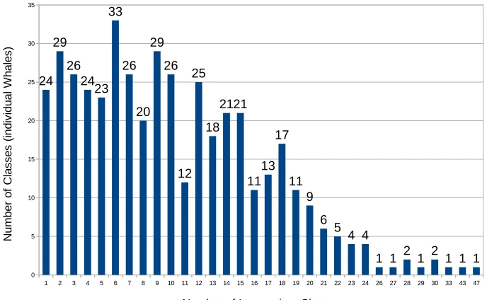
The number of whales in each individual whale varies significantly from whales with 1 training image up to 47 training images. Figure 2.8 shows a summary of the number of whales with a certain number of images. For instance, there are 24 whales (or classes) with only 1 training image and 29 whales with 2 training images. On the other hand, there is 1 whale with 47 training images. The average number of training images in each class is 10 training images. We developed our model on a laptop equipped with GTX980M (4GB) graphics card. Only 3.5GB of GPU RAM was available for training. The code was developed using Theano [2, 4] which is a python library for optimizing and evaluating mathematical expressions in multidi-mensional arrays. We also used keras [9] which is a highly modular library to train neural networks on GPUs or CPUs.

In order to pre-process the image data and to perform geometric transformations, we used scikit-image [83] and openCV [6]. The networks were trained in batches of size 32 images. This is the largest batch size we could fit in the GPU memory. The CPU performs data aug-mentation on each batch before sending it to the GPU for training.

(42)

2.6. Implementation andResults 29

1 2 3 4 5 6 7 8 9 10 11 12 13 14 15 16 17 18 19 20 21 22 23 24 26 27 28 29 30 33 43 47 0 5 10 15 20 25 30 35 24 29 26 24₂₃ 33 26 20 29 26 12 25 18 2121 11 13 17 11 9 6 ₅ 4 4

1 1 2 1 2 1 1 1

Number of Images in a Class

N um be r of C la ss es ( in di vi du al W ha le s)

Figure 2.8: A summary of the number of whales with a certain number of images. There are 24 whales (or classes) with only 1 training image and 29 whales with 2 images. On the other end of the chart, we can see that there are few classes with a relatively high number of training images. For instance, there is one whale with 47 training images.

The metric used by the server to evaluate the predictions is the multi-class logarithmic loss (also known as categorical cross-entropy). The equation for this metric is:

logloss= −1 n

N X

i=1

M X

j=1

yi jlog(pi j) (2.6)

where N is the number of images in the predictions file (or the number of images in the test set), M is the number of labels (the total number of individual whales). yi j is a mapping from

the imageito the true label j(for example,yi j is 1 if the imageibelongs to the whale jand 0

if it does not). log(pi j) is the natural log of the predicted probability made by the model that

the imageibelongs to whale j.

(43)

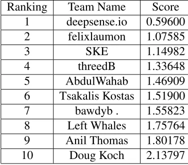
Table 2.2: Teams Ranking: this table shows the ranking of the solution we describe in the paper. The solution ranked in the 5thposition. The table only shows the top 10 teams while the number of teams that participated in the competition is 364. The full table can be found on the web page of the competition [43]

Ranking Team Name Score 1 deepsense.io 0.59600 2 felixlaumon 1.07585 3 SKE 1.14982 4 threedB 1.33648 5 AbdulWahab 1.46909 6 Tsakalis Kostas 1.51900 7 bawdyb . 1.55823 8 Left Whales 1.75764 9 Anil Thomas 1.80178 10 Doug Koch 2.13797

On the server, the log loss score we achieved is 1.47. The top-1 accuracy of the module on the validation set is 69.7% while the top-5 predictions accuracy is 85.0%.

We used the same loss function to train the localization modules. Figure 2.9 show the train and validation log loss progress for both the bonnet localization network and the blow hole network, respectively. In Figure 2.9, we can see that the loss function of the bonnet localization network decreases from 4.5 to around 2.28 at the end of training.

As shown in Figure 2.9, the blow hole localization loss decreases from 5 to around 2.52 at the end of the training. The performance of the bonnet network is slightly better than the blow hole localization network as the former has a lower loss than the latter. This is likely because for many samples the blow hole is completely covered by water (white pixels) while the bonnet is visible in most of the images.

Figure 2.9 also shows the performance of loss function of the head localization network. The loss value goes down from 5.03 to around 3.87. Because both the validation and training losses curves are very close to each other, the performance may be improved slightly by using a larger network.

(44)

0 ₂0 ₄0 ₆0 ₈0

1 0 0 1 2 0 1 4 0 1 6 0 1 8 0 2 0 0 2 2 0 0 0.5 1 1.5 2 2.5 3 3.5 4 4.5 5 4.0249 2.7627 2.39272.36882.32882.29292.30202.29062.26162.27652.2843

Bonnet Localization Loss Training Loss Validation Loss Epochs L o g L o ss

0 ₁₀ ₂₀ ₃₀ ₄₀ ₅₀ ₆₀ ₇₀ ₈₀ ₉₀

10 0 11 0 12 0 13 0 14 0 15 0 16 0 17 0 18 0 19 0 20 0 21 0 22 0 0 1 2 3 4 5 6 3.9253 3.1302

2.6767 2.5897 2.5368 2.5261 2.5383 2.5272 2.5247

Blow Hole Localization Loss

Training Loss Validation Loss Epochs L o g L o ss

0 ₁₀ ₂₀ ₃₀ ₄₀ ₅₀ ₆₀ ₇₀ ₈₀ ₉₀

10 0 11 0 12 0 13 0 14 0 15 0 16 0 17 0 18 0 19 0 20 0 21 0 22 0 0 1 2 3 4 5 6 5.0336

4.07193.95623.92653.90233.88833.8748 3.87123.8705 3.87573.8685

Head Localization Loss

Training Loss Validation Loss Epochs L o g L o ss

0 ₂₀ ₄₀ ₆₀ ₈₀

10 0 12 0 14 0 16 0 18 0 20 0 22 0 24 0 26 0 28 0 30 0 32 0 34 0 36 0 38 0 40 0 42 0 44 0 0 1 2 3 4 5 6 7 6.07 _5.87 4.80 3.45 2.99 _2.72 2.26 _2.11

1.99 1.91 _{1.79 1.63}

Recognition Loss

Training Loss Validation Loss

Epochs L o g L o ss

Figure 2.9: Loss Curve: This figure shows the training and validation loss during the training of the four deep learning models (bonnet localization model, blow hole model, head localization model, and whale recognition model.)

useful to track the quality of the localization visually. Figures 2.10 and 2.11 show a random set of images of localized whales bodies and localized whale heads, respectively.

(45)

Figure 2.10: A sample of localized whale bodies.

Figure 2.11: A sample of localized whale heads. same manner when training the blow hole and head localization networks.

As we mentioned earlier, using a multi-stage approach was the only way to be able to train a deep learning model on this data set. However, when carrying out a multi-stage approach, there is a risk of error propagating from one stage to the next. Figure 2.13 shows a sample of cases where the whale body crops could not be localized correctly. In the images shown in this Figure, some of them do not show the full callosities pattern on the whale head while other include the whale body oriented in the wrong directory. There are approximately 0.7% of cases where the model could not correctly localize the body.

The head localization error is higher than the body localization error. The head localization error is 2.9%. Figure 2.14 shows a sample of images where the head was not localized correctly. These images include cases where the callosities pattern is not fully shown in the image.

(46)

Predicted Location True Location

0 5 10 15 20 25 30 35

Figure 2.12: This figure shows how the network performance in tracking the location of the bonnet improves as it is being trained. At epoch 0, the network predicts the location of the bonnet to be in the middle of the image. Later, the network gradually becomes capable at predicting the location of the bonnet.

Figure 2.13: A sample showing cases where the body of the whale was not localized correctly. In the images shown in this Figure, some of them do not show the full callosities pattern on the whale head while other include the whale body oriented in the wrong directory.

Equation 2.7:

IoU = Mtrue∩Mpred Mtrue∪Mpred

(2.7) where Mtrue, Mpred are the true and predicted masks. On the validation set, the average body

(47)

Figure 2.14: A sample showing cases where the head of the whale was not localized correctly. These images include cases where the callosities pattern is not fully shown in the image.

2.7 CONCLUSION

We introduced a method to recognize individual whales from the callosities on their head. This method can help in the conservation efforts of marine biologists. Because the size of the available training images is very low, overfitting is very difficult to avoid. In fact, we could not achieve an accuracy of more than 8% when training a deep learning model to classify the whales directly. We solved this problem by introducing a model to localize the head of the whale and training the recognition model on it. This helps the recognition model to focus on the callosities features located on the head of the whale. Our model’s top-1 and top-5 predictions accuracies are 69.7% and 85%, respectively. We strongly believe that the performance can be boosted by increasing the size of the training set. In addition, improving the body and head localization models will likely improve the whale classification error.

(48)

Chapter 3 Right whale Recognition using the Wide

Localization Network

3.1 Introduction

In the previous chapter, we described how the Right whale recognition problem can be solved by localizing the bonnet and blow hole using the standard localization network. In this chapter, we will improve the results by using the wide localization network. Furthermore, after orient-ing the heads towards the east, we will localize three points on the of the whale. Then, these points will be used to slightly rotate the head to make sure that the angle with the x axis is exactly 0. In addition, these three points will be used to extract the region of interest.

3.2 Method Overview

Training the recognition model on the raw images is unlikely to yield good results. When training the recognition model on the original images, we could not achieve good results due

0_{The majority of this chapter was originally published in: AbdulWahab Kabani, and Mahmoud R. El-Sakka}

“Improving Right whale Recognition by Fine-tuning Alignment and Using Wide Localization Network”, Cana-dian Conference on Electrical and Computer Engineering (CCECE), Windsor, Canada, May 2017 [pre-print]. [40]

(49)

Input Image And Head Mask

1% 90% ... 2%

Whale IDs Probability Distribution

Localize Head Localize Bonnet

and Blow hole

Localize region of interest using 3 points Train

Head Localizer

Train Bonnet and Blow hole Localizer

Train Traingle Points

Localize Region of Interest and fine alignment Orient the

whale

Input Image And Two points Mask

Train Classifier

Head Localization Bonnet and Blow hole Localization

Head Orientation and Region of Interest Alignment Recognition

Figure 3.1: The overview of the method: the first stage involves performing head localization. The second stage involves identifying the bonnet and blow hole. Using these two points, the head is oriented east. In stage 3, we perform further fine tuning alignment and a bounding box is extracted. Once the region of interest is identified, the region of interest is passed to the recognition network to predict the ID based on the callosities pattern.

(50)

3.3. HeadLocalization 37

what was suggested in [5]. However, we used a different localization network called wide net. The main advantage of this network is that it has the ability to predict region of interests with different shapes (rectangles, circles, or any arbitrary shaped region of interest). In addition, it has a low memory requirement making it ideal for use as a pre-processing step.

In the second stage, a wide net model is trained to localize the bonnet and blow hole. As suggested in [82], we use these two points to orient the head in one direction. In the third stage, we train a wide net model to predict three points (bonnet and two points representing the post blow hole callosities). These points are used to perform further fine-tuning alignment. In addition, we can use them to extract a very tight bounding box that only shows the most discriminative features.

Once a bounding box is extracted, it is used to train an ensemble of deep learning models to classify and identify each image. What is unique about our solution is that we use deep learning model called the wide net, which we will describe in Section 3.3. In addition, we perform an extra fine-tuning step after head orientation using three support points.

3.3 Head Localization

(51)

(3, h, w) C on v (5 ,5 ) C on v (5 ,5 ) C on v (3 ,3 ) C on v (3,3 ) C on v (3 ,3 ) C on v (3 ,3 ) C on v (3 ,3 ) C on v (3 ,3 ) C on v (3 ,3 ) C on v (3 ,3 ) C on v (3 ,3 ) C on v (3 ,3 ) C on v (3 ,3 ) C on v (3 ,3 ) C on v (3,3 ) C on v (3 ,3 ) C on v (3 ,3 ) C on v (3 ,3 ) C on v (3 ,3 ) C on v (3 ,3 ) In pu t

(32, h, w) (64, h/2, w/2) (128, h/4, h/4) (256, h/8, h/8) (512, h/16, h/16)

Block_1 Block_2 Block_3 Block_4 Block_5

Upsample Blocks (3,4,5) & Merge blocks (2,3,4,5)

(128, h/4, w/4) (64, h/2, w/2)

Upsample Blocks (4,5)

& Merge blocks (3,4,5) & Merge blocks (4,5)Upsample Block (5)

Conv (5,5)

Conv (5,5) Conv (5,5)

Upsample & Merge

(256, h/8, w/8)

Conv (5,5) Output

(32, h, w)

(oc, h, w)

L ev el _1 L evel _2 L evel _3 G ro u p _1 G ro u p _2 G rou p _3

Figure 3.2: The architecture of wide net: the network is composed of three levels. Level 1 is just like any typical recognition network. Level 2 involves merging the last layer from each block in level 1 in three different ways. Finally, in level 3, the outputs of level 2 are combined and a mask is produced. Abbreviations: h is the height of the image, w is the width of the image, oc is the output channel size.

The last layer in the network has a sigmoid activation to map the pre-activation values into values between 0 and 1. Rectified linear units (ReLU) activation [61, 30] is used after each layer. Each pre-activation is followed by batch normalization [36]. In order to extract more abstract features, we use Max-pooling in level 1. As a result, the layers in each block in level 1 will have different sizes. In order to combine them together in level 2, we use upsampling to ensuring that the layers can be merged. This network has a low processing footprint and was previously tested on a device with only 3.5 GPU memory.

(52)

3.4. Bonnet andBlowHoleLocalization 39

resized to 128(height)×192(width). The ground truth for this network involves a mask that contains zero pixels everywhere except in the region of interest.

Because we are using a sigmoid activation in the output layer, our loss function is binary cross-entropy. The learning rate was set at 0.001 and decreased by 50% if the validation error does improve after 20 epochs. The head localization model is trained for 100 epochs. After that, we use it to predict the bounding box for the whale head. We are now ready for the bonnet and blow hole localization.

3.4 Bonnet and Blow Hole Localization

The bonnet and blow hole localization stage (shown in Figure 3.1) involves training a deep learning model to locate the two points. This was proposed in [82] as a means to speed up the training process. We also noticed that it is useful in reducing the amount of pixels that represent the surrounding water. These pixels can lead to overfitting because the training set is not large enough. Therefore, the model may be tricked into thinking that these pixels influence the kind of target we are interested in.

The training process and network architecture (Figure 3.2) is exactly the same as we de-scribed in Section 3.3. However, the input images were resized into 128(height)×128(width). In addition, this network will output a mask with 2 channels. One channel produces the location of the bonnet while the other channel predicts the location of the blow hole.

Once these two points are localized, we can easily rotate the images. This is because the angle of the whale with respect to the xaxis can be estimated by Equation 3.1.

θ=tan−1(ybonnet−yblowHole

xbonnet−xblowHole

(53)

width

he

ig

ht

Figure 3.3: Three points are detected: the bonnet and two points representing the post blow hole callosities. The post blow hole callosities points can be used to extract the height of the region of interest. The bonnet and the average of the post blow hole callosities points are used to get the width and perform fine alignment by rotating the image if the angle with the horizon is more than 1 degree.

Improving Deep Learning Image Recognition Performance Using Region of Interest Localization Networks

Scholarship@Western

Scholarship@Western

Improving Deep Learning Image Recognition Performance Using

Improving Deep Learning Image Recognition Performance Using

Region of Interest Localization Networks

Region of Interest Localization Networks

Abstract

Co-Authorship Statement

Contents

List of Appendices

Chapter 1

Introduction

1.1

The Deep Learning Journey

1.2

Region of Interest Localization

1.3

Right whale Recognition

1.4

Left Ventricle and Ejection Fraction Estimation

Chapter 2

Right whale Recognition using the

Standard Localization Network

2.1

Introduction

2.2

Method Overview

2.3

Body Localization

2.4

Head Localization

2.5

Recognition

2.6

Implementation and Results

2.7

CONCLUSION

Chapter 3

Right whale Recognition using the Wide

Localization Network

3.1

Introduction

3.2

Method Overview

3.3

Head Localization

3.4

Bonnet and Blow Hole Localization

width

he

ig

ht

3.5

Head Orientation and Region of Interest Alignment