Modelling of Electric Field Strength Amplification at the Tips
of Thin Conductive Rods Arrays
Marina Rezinkina*
Abstract—Degree of the electric field (EF) amplification at the tips of thin and long conductive rods array has been calculated. It is shown that such amplification depends on the rods height (H) and radius (R), as well as on the distance between separate rods in the array. For simulation, an approach to numerical calculation of the EF near conductive rods with a large ratio of height to radius:
H/R > 102–104 has been proposed. Rods with such parameters may represent carbon nanotubes, channels of breakdowns in insulation, lightning leader channels, lightning rods, etc. The proposed approach is based on the finite integration technique. It also uses the analytical law of decrease of the EF strength and potential of a conductive ellipsoid under potential in the directions perpendicular to the ellipsoid axis and above its tip. As a result, numerical calculations of the EF distribution in systems with such rods were carried out applying calculation grids with steps proportional to the rods length, not their diameters. It permits substantial decrease of the required computational resources such as memory and time.
1. INTRODUCTION
In some problem solutions, information on the electric field (EF) distribution in systems with objects that can be represented as thin and long conductive rods is required. Examples of such systems are leader channels of lightning, lightning rods, and channels of incomplete breakdowns in insulation [1, 2]. The cases when a ratio of the rods height (H) to their radius (R) can reach 102–104and more are considered. Another area of such problems’ application is the emission devices using arrays of carbon nanotubes (CNTs) [3–5]. According to [6], the problem of determination of the EF strength amplification at the tips of the CNT array: β =Emax/E0 (whereEmax is maximum EF strength at the rods tips, andE0 is the average applied EF strength), depending on their parameters, is not completely solved despite that it has been considered in many researches.
In many cases, usage of the analytical methods for obtaining the EF distribution in such systems is not possible, so numerical methods should be applied. With regard of a large rods’ length and their small radius, usage of the numerical methods of equivalent charges [7] or integral equations [8, 9] would be necessary for calculating an extremely large number of unknown charges located on the rod axis, because distances between such charges should be comparable with the rod radius and not with its length. Application of the finite element method [10] would be excessive, as the considered systems as a rule include straight objects. Therefore, usage of the finite difference methods seems most appropriate. At this, a problem of choice of the value of computational grid step Δ arises. In the classical approach to the finite-difference methods usage, Δ should not be bigger than the rod radiusR. So, in 3-D problems calculation in systems with the rods havingH/R >102–104, solution of systems of equations of a rather large order is necessary, and, at this, as practice has shown that significant errors can accumulate.
Received 27 October 2019, Accepted 23 December 2019, Scheduled 10 January 2020 * Corresponding author: Marina Rezinkina (maryna.rezynkina@gmail.com).
To calculate the EF near an infinitely long thin conductive cylindrical rod by the finite difference method, an approach that uses the known law of the EF strength decrease in the directions perpendicular to the rod axis as an inversely proportion function from distance to it can be applied [11]. Grid step Δ can be significantly bigger than the rod radius. With presenting a rod as a uniformly charged filament, this method was applied also to rods of finite length [12, 13]. However, in such an approach, the relative errors less than 5% of the EF potentials calculation are achieved only on a certain distance from the rod tip, and the error of the EF strength determination can be much bigger. It is caused by the used assumption that charge is distributed evenly along the rod axis, which is not correct for the rod’s tip. To solve this problem, with obtaining the coefficients of final difference equations for the nodes surrounding the rod, the analytical expressions for the EF of a conductive elongated spheroid upon electric potential can be used instead of traditional one for final difference methods linear law of potentials changing. The aim of the work is numerical investigation with the help of such an approach of influence of the parameters of the rods array, for example used in the emission devices, on a degree of the EF strength amplification at the rods’ tips.
2. CALCULATION OF THE EF IN SYSTEMS WITH CONDUCTIVE RODS
A system containing a grounded conductive rod located in the homogeneous EF with strength E0 is considered. For EF calculation, the finite integration technique [14, 15] was used. This method supposes integration of the solvable equations over the volumes or surfaces of the unit cells into which the studied area is divided. Usage of this method allows automatically taking into account conditions on the boundaries of inhomogeneous media as well as nonlinear dependence of the electric field parameters between adjacent nods of the computational domain.
The computational domain was divided into parallelepiped unit cells having volume V in such a way that the nodes of the computational grid (i,j,k), in which the electric potentials are determined, lie on the interfaces of the media and on the conductive rod axis (see Fig. 1).
Y
Z X
i, j+1, k-1 i+1, j+1, k-1
i+1, j, k-1
i+1, j, k i, j, k-1
i, j+1, k
i , j , k
i , j -1, k i-1, j, k
i, j, k+1
1 ΔZk S Sxz
j
ΔY
i
ΔX Syz
r r r
r r Sxy
r
i+1, j+1, k 2
(a) (b) (c)
Figure 1. Calculated system. 1 is conductive rod. (a) Separate rod at application of the EF with strength E0; (b) single rod in the rods array at application of the EF with strength E0; (c) cell of the calculation scheme. ΔXi = ΔYj = ΔZk= Δ — grid step.
The solvable equation was obtained by divergence operation application to Maxwell equation [16]
rot ¯H=γE¯+∂D/∂t,¯ (1)
of Eq. (1) is equal to zero. So we get:
S
γEnds= 0, (2)
wheren is normal to the surfaceS comprising volume V.
By expressing EF strength through electric potential ϕ: ¯E = −gradϕ, the solvable equation is
written as follows:
S
γi, j, k
−∂ϕ
∂n
ds= 0, (3)
whereγi, j, k is the relative specific conductivity of the (i, j, k)-th cell.
It is considered that the vertices of the (i, j, k)-th cell are the following nodes: (i, j, k), (i, j+ 1, k), (i, j, k+1), (i, j+1, k+1), (i+1, j, k+1), (i+1, j+1, k), (i+1, j, k), (i+1, j+1, k+1) (see Fig. 1(c)). Due to integration operation over the cell volumes, boundary conditions on the media interfaces are satisfied automatically, and no additional equations are required. Eq. (2) is written for each computational grid node.
An assumption that values of the sought electromagnetic field parameters change linearly between neighboring nodes of the computational grid is used as a rule in finite difference methods [11]. However, in the immediate vicinity of a conductive rod, this assumption is possible only when a spatial step Δ is not larger than the rod radius. As noted above, usage of such a fine 3D grid for determination of the electric field parameters in the vicinity of the rods with H/R > 102–104 causes calculation errors accumulation. To solve this problem, the following approach is used.
The nodes located on the conductive rod axis are designated by index “r”: (ir, jr, kr) (see Fig. 1(c)). In this case, specific conductivity between (ir,jr,kr) nodes in the direction of the rod axis (in our case axis OY, see Fig. 1) is supposed to be equal to specific conductivity of metal from which the rod is made — γR. As the grid step is chosen proportional to the height of the rod, i.e., Δ R,
nonlinear dependence of the EF strength and potential takes place mainly in the region between the nodes (ir, jr, kr) and the nodes adjacent to them in the radial direction, and also between a node located on the rod tip (it is denoted asir,jrmax,kr) and a node above it — (ir,jrmax+ 1,kr). In such a case, it is convenient to present conductivity in Eq. (3), which characterizes the electrical parameters, including those around the rod, in the form of a tensor:
γi, j, k=
⎡
⎣ γi, j, k0·kx γi, j, k0·ky 00
0 0 γi, j, k·kz
⎤
⎦, (4)
where kx, ky, kz are coefficients equal to 1 for all nodes except kx and kz for nodes (ir, jr, kr), (ir − 1, jr, kr), (ir, jr, kr −1) and ky for node (ir, jrmax, kr); ky = πR2/Δ2 for (ir, jr, kr) nodes;
γir, jr, kr =γR.
Eq. (3) is rewritten as follows:
S
−
γi, j, k∂ϕ∂ndS = 0. (5)
To find coefficients kx, kz, ky in Eq. (4), ϕ and EF strength components in the vicinity of the
rod are written with the help of the analytical expressions for an elongated conductive spheroid under potential U0 with small semi-axes equal toR and large semi-axis equal to H [16]:
ϕ(xi, yj, zk) = U0·fϕU(xi, yj, zk); (6)
Ex(xi, yj, zk) = U0·fUEx(xi, yj, zk); (7)
Ey(xi, yj, zk) = U0·fUEy(xi, yj, zk); (8)
Ez(xi, yj, zk) = U0·fUEz(xi, yj, zk), (9) where
fϕU(xi, yj, zk) = 2 ln(21
H/R) ·ln
ξ+H2+√H2−R2
fUEx(xi, yj, zk) = −fUE(xi, yj, zk)·dξxz(xi, yj, zk)·xi;
fUEy(xi, yj, zk) = −fUE(xi, yj, zk)·dξy(xi, yj, zk)·yj;
fUEz(xi, yj, zk) = −fUE(xi, yj, zk)·dξxz(xi, yj, zk)·zk;
fUE(xi, yj, zk) = −2 ln(21H/R) ·
√
H2−R2
ξ+H2·(ξ+R2);
dξxz(xi, yj, zk) =
1− p−H 2
p2−q
; dξy(xi, yj, zk) =
1− p−R 2
p2−q
;
ξ = −p+ p2−q; ξ >−R2 [16];
p = H
2+R2−x2
i +yj2+zk2
2 ; q =H
2
R−H2(x2i +zk2)−R2yj2;
xi, yj,zk are Cartesian coordinates of (i, j, k)-th grid node; Ex,Ey, Ez arex,y, z components of the
EF strength.
By analogy of the common usage of finite difference methods, derivative fromϕin Eq. (5) is written in the form of difference of the potentials in the node on the rod axis and in the node located from it in the radial direction on a distance of computational grid step Δ. It is assumed that potentials of (ir, jr, kr) nodes belonging to the rod are equal to U0, and potentials in the nodes one step apart from the rod axis can be represented as Eq. (6). Then
∂ϕ/∂x|x=xir+1≈Δϕ/Δ = [ϕ(xir, yjr, zkr)−ϕ(xir−1, yjr, zkr)]/Δ =U0·[1−fϕU(xir−1, yjr, zkr)]/Δ, (11) wherefϕU(xi, yj, zk) — see Eq. (10).
U0can be expressed from Eq. (11) through Δϕ/Δ with regard of nonlinear change of corresponding potentials as follows:
U0 = Δϕ
Δ ·Dx, (12)
whereDx= 1−fϕU(xir−Δ1,yjr,zkr).
Eq. (7) is written forx=xir+1/2 =xir+ Δ/2 — coordinate of one ofS surfaces perpendicular to
OX axis, which is located on distance Δ/2 from the rod axis and over which integration over a unit cell
V is performed (see Fig. 1(c) —Syz). U0 is substituted in Eq. (7) as Eq. (12):
Ex(xir+1/2, yjr, zkr) = Δϕ
Δ ·KEx(xir+1/2, yjr, zkr), (13) whereKEx(xir+1/2, yjr, zkr) =Dx· |fUEx(xir+1/2, yjr, zkr)|.
Other EF strength components are written in the same way. Then each EF component is substituted in the left-hand side of Eq. (2) and integrated over surface S. For instance,Ex in the form of Eq. (13)
is substituted in Eq. (2) and integrated over surfaceSyz. (see Fig. 1(c)). As a result, an expression for
the coefficient kx in Eq. (4), defining nonlinear character of the EF change between two nodes, one of
which is located on the rod axis, and the other is located on a distance of one spatial step from it in the radial direction, is written as follows:
kx(xir, yjr, zkr) =
yjr+Δ/2
yjr−Δ/2
zkr+Δ/2
zkr−Δ/2
KEx(xir+1/2, yjr, zkr)dydz. (14)
help of similar transformations:
kz(xir, yjr, zkr) =
yjr+Δ/2
yjr−Δ/2
xir+Δ/2
xir−Δ/2
KEz(xir, yjr, zkr+1/2)dydx; (15)
ky(xir, yjrmax, zkr) =
zkr+Δ/2
zkr−Δ/2
xir+Δ/2
xir−Δ/2
KEy(xir, yjrmax +1/2, zkr)dzdx, (16)
where KEy(xir, yjrmax +1/2, zkr) = Dy · |fUEy(xir, yjrmam+1/2, zkr)|; KEz(xir, yjr, zkr+1/2) = Dz ·
|fUEz(xir, yjr, zkr+1/2)|;Dz = 1−fϕU(iΔr,jr,kr−1);Dy = 1−fϕU(ir,jΔrmax +1,kr).
The considered computational domain belongs to the so-called open ones. To reduce its size, uniaxial perfectly matched layers (UPML) are placed on its boundaries [11, 17]. Conductivity in these layers is assumed being a tensor in the form of Eq. (4), whose components vary along the layer depth
daccording to the exponent law. Thus, in the direction ofOY axis:
fy = 1 + (fmax−1)·[|y|/d]m >1,
where fmax is the maximum value offy on the outerUPML boundary; m is the degree of exponent; y is the coordinate.
For UPML layers, coefficients kx, ky, kz, which determine components of the conductivity tensor
in Eq. (4), are assigned equal to 1/fx, 1/fy, 1/fz in the direction perpendicular to the layer, and equal
to fx, fy,fz in the directions parallel to the layer. To find the EF parameters, a system of equations
relatively unknown potentials in the finite difference form consisting of Equation (5) written for each node of the calculation domain is solved. For this, the iterative method of variable directions and the sweep method are used. Implementation of these methods is described elsewhere [18, 19].
3. EVALUATION OF ACCURACY OF CONDUCTIVE ROD EF CALCULATION
To assess accuracy of the described method, EF numerical calculation is carried out in test systems with following parameters: first — the uniform EF with strength E0 = 1 V/µm is applied to a conductive rod with height H = 10µm and radius R = 5 nm located on the surface of grounded semi-plane having zero y coordinate, second — potential U0 = 1 V is applied to the conductive rod. EF in such systems can be described analytically [16]. Computational grid step at numerical calculations is chosen equal to Δ = 1µm; computational domain dimensions are as follows (see Fig. 1(a)): xmin =−10µm,
xmax = 10µm, ymin = 0, ymax = 20µm, zmin = −10µm, zmax = 10µm (zmin, zmax are minimal and maximal values of coordinates in the azimuthal direction). In the first test system, conditions unperturbed by the conductive rod presence are assigned on the boundaries of the computational domain as follows: ∂ϕ/∂x = 0 at x = xmin, x = xmax; ∂ϕ/∂z = 0 at z = zmin, z = zmax; ϕ = 0 aty = 0;∂ϕ/∂y=−E0·fmaxat y=ymax. The last condition permits assigning level of the applied EF strength equal toE0, as on theUPML outer boundary∂ϕ/∂y is assigned in fmax times bigger. In the second test system, conditions for ϕ on the computational domain boundaries are assigned as follows:
∂ϕ/∂y= 0 fory= 0, except for a node where the rod base is located (coordinates x= 0,y= 0, z= 0) — ϕ = U0; ∂ϕ/∂x = 0 at x = xmin, x = xmax; ∂ϕ/∂z = 0 at z = zmin, z = zmax. In both systems
UPMLhaving N = 10 layers withm= 3, fmax= 300 [11] are placed on the domains outer boundaries. The modulus of electric field strength is calculated by averaging itsx-th,y-th, andz-th components over a cell volume:
|En(xi, yj, zk)|=
E2
x(xi, yj, zk) +Ey2(xi, yj, zk) +Ez2(xi, yj, zk),
where Ex(xi, yj, zk) = 0.25 · [(ϕi+1,j,k − ϕi,j,k) + (ϕi+1,j+1,k − ϕi,j+1,k) + (ϕi+1,j,k+1 − ϕi,j,k+1) + (ϕi+1,j+1,k+1 −ϕi,j+1,k+1)]/Δ]; Ey(xi, yj, zk) = 0.25 · [(ϕi,j+1,k −ϕi,j,k) + (ϕi+1,j+1,k −ϕi+1,j,k) + (ϕi,j+1,k+1−ϕi,j,k+1)+(ϕi+1,j+1,k+1−ϕi+1,j,k+1)/Δ];Ez(xi, yj, zk) = 0.25·[(ϕi,j,k+1−ϕi,j,k)+(ϕi,j+1,k+1−
As analytical solutions, expressions for the EF potential and strength of an elongated conductive spheroid [16] are used. Relative errors of the EF potential (δui, j, k) and EF strength (δei, j, k) calculation
are determined as follows:
δui, j, k =|ϕni, j, k| − |ϕani, j, k|
/|ϕan
i, j, k|; δei, j, k =|Ei, j, kn | − |Eani, j, k|/|Eani, j, k|,
where|Eni, j, k|,|Eani, j, k|are numerical and analytical values of the EF strength modulus in (i, j, k)-th cell center, and|ϕni, j, k|,|ϕani, j, k|are numerical and analytical values of the EF potential in (i, j, k)-th node.
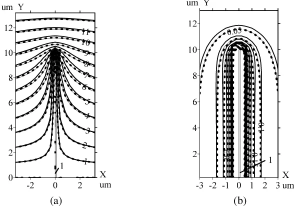
Figure 2 shows distributions of lines of equal potential (a) and equal EF strength (b) calculated using analytical expressions for an elongated conductive spheroid (shown by dashed lines), as well as such levels calculated using the described above method (shown by solid thin lines). This figure also shows distributions calculated in accordance with [12] (solid bold lines). In calculation in accordance with [12], maximum errors levels are equal to δeUmax ≈19.7% for the first system and δeUmax ≈ 45.6% for the second system. As from carried calculations, finding by (14)–(16) kx, ky, kz (see (4)), which represent coefficients of final difference equations for nodes around the rod, the relative errors maximum values observed in the region around rod’s tip are as follows: δeEmax≈2%,δuEmax≈1.8% for the first test system and δeUmax ≈6.54%, δuUmax ≈ 9.87% for the second test system. However, the maximum error for the second test system is only in the region adjacent to the rod’s tip, and in the rest region it is less than 3%. Calculations performed for the test systems show that twofold decrease of the computational grid step and twofold increase of grid dimensions do not cause the EF distributions change within the assigned relative error — 3%.
(a) (b)
Figure 2. Calculated distributions of the equal potential lines (in V) at application of the uniform EF with (a) strength E0 = 1 V/µm to the rod and (b) equal EF strength (in V/µm) in case of U0 = 1 V potential application to the rod. 1 is rod. — — numerical calculation in accordance with the described method; — numerical calculation in accordance with the method described in [12]; — analytical solution for the rod presentation as an elongated conductive spheroid [16].
4. CALCULATION OF DEGREE OF THE EF STRENGTH AMPLIFICATION AT THE TIPS OF CONDUCTIVE RODS ARRAY DEPENDING ON THEIR
PARAMETERS
as their high electric conductivity. For the effective operation of the cold field emission cathodes, it is necessary to increase density of CNTs location in their array. However, in this case, the EF strength decreases at the nanotubes tips because their screening by neighboring closely located CNTs should be taken into account. In a number of researches, dependence of the CNT emission current on amplification factor of the EF strength at their tips β = Emax/E0 was studied [3–6]. However, the data of various authors on the quantitative dependences of the CNTs characteristics on their parameters do not always coincide [20]. In [21], the calculation results for choosing the optimal parameters of the cold field emission cathodes on CNTs were presented, and influence ofH/R ratio on functionβ =f(S/H) (where
S is the distance between the CNTs) was not taken into account, as all calculated dependences of β
on S at various values of H and R can be presented as one dependence β = f(S/H) (β for different
H and R coincide at the same S/H). In [3], the calculated and experimentally obtained dependences
β =f(S/H) were given for one H/R ratio.
To evaluate effect of the CNT height to radius ratio on dependence β = f(S/H), a series of calculations is performed using the above described method. The investigated calculation system is shown in Fig. 1(b) (Δ = 0.2µm). As the greatest decrease of the EF strength because of screening occurs at the tips of the rods located inside the array and not on its fringes, the EF is calculated for such a rod. It is assumed that coordinates of a base of the investigated rod are: x = 0, y = 0, z = 0 (see Fig. 1(b)). To consider the EF in the case of an array of identical rods withH = 5µm located on distancesS from each other, symmetric boundary conditions on the computational domain boundaries surrounding a single rod (xmin =−S/2,xmax=S/2,zmin =−S/2, zmax=S/2) are used: ∂ϕ/∂x = 0 at x=xmin,x=xmax;∂ϕ/∂z = 0 atz=zmin,z=zmax. The boundary conditions fory are as follows:
ϕ= 0 at y = 0, ∂ϕ/∂y =−E0·fmax at y = ymax (ymax = 10µm). UPML parameters are as follows:
N = 10, m= 3,fmax= 300. Levels of S are varied in the range: 2.5–7.5µm, and levels ofR are varied in the range: 6–50 nm.
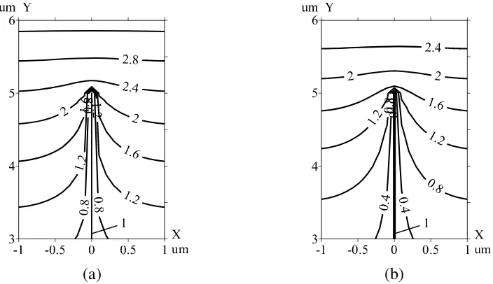
Figure 3 shows results of calculation of the lines of equal potential in the zone surrounding the rod at the EF with strength E0 =1 V/µm application. These calculations are performed for two CNT arrays having the sameS = 2.5µm, H = 5µm but different CNT radii: R= 1 nm (a) and R = 25 nm (b). As can be seen from these dependences, with increase of R, more significant decrease of the EF strength above the CNT tip occurs, which should be taken into account at the choice of CNT arrays parameters.
There are experimental data on the degree ofβ reduction with respect toβ0 (whereβ0=Emax/E0
X
um 3-1 -0.5 0 0.5 1
4 5 6
(a) (b)
Figure 3. Calculated distributions of the lines of equal potential (in V) in the vicinity of a CNT with height H = 5µm, located in an array of rods spaced apart on distance S = 0.5·H at the uniform EF with strength E0 = 1 V/µm application. 1 is rod. (a) CNT radius R = 1 nm, (b) CNT radius
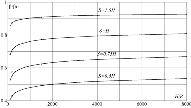
isβvalue for a separate rod without rods array — see Fig. 1(a)) in dependence on the ratio between rods distances (S) and their height (H) atH = 5 mm, R= 25 nm [3]. Comparison of these data (see in Fig. 4) with computation results obtained with the help of the described model shows their coincidence within 1–3%.
Figure 4 shows calculated dependences ofβ/β0 onH/R at various distances between the rods (S). As can be seen from the curves comparison, the smaller the S is, the greater the H/R influence is on the degree of β/β0 reduction. At S = 0.5·H, range ofβ/β0 increase is 32% when H/R changes from 100 to 8000; at S = 0.75·H such a range is 27%; at S =H it is 18.5%; at S = 1.5·H it is 8.3%. At
H/R >4000, differences of β/β0 levels are no more than 3%.
Figure 4. Calculated dependences of β/β0 on the CNT height to radius ratio (H/R) for various distances between CNTs in their array (S). — data from [3].
5. CONCLUSION
A method for EF calculation in systems with conductive rods is proposed. It allows determination of the EF distribution at the step of the computational grid proportional to the rod height, and not to its radius. Differences from analytical solutions for a separate rod located in the applied EF do not exceed 2%. This approach is applicable to the EF calculation of rods array with considering the EF of one CNT and introducing symmetric boundary conditions of the type ∂ϕ/∂n = 0 on the lateral computational domain boundaries. Usage of this technique provides a possibility to evaluate influence of the rods height to radius ratio on the degree of the EF strength decrease at their tips in the CNT array because of electrostatic shielding. At H/Rof the order of 100–200, decrease ofβ/β0 (the ratio of the EF strength maximum level at the rods tips to the applied EF strength (β) versus the same levels for the rod without an array (β0)) can be up to 32% with respect to the rods withH/R of the order of 2000–4000, which should be taken into account at choice of parameters of the cold field emission cathodes on CNTs.
REFERENCES
1. Cooray, V., Lightning Protection, The Institution of Engineering and Technology, London, 2010. 2. Bazelyan, E. M. and Yu. P. Raizer, Lightning Physics and Lightning Protection, IOP Publishing,
Bristol, 2000.
PECVD for customized compact field emission devices to be used in X-ray source applications,”
Nanomaterials, Vol. 8, 378-1–378-9, 2018.
5. Bocharov, G. S., A. V. Eletskii, and S. Grigory, “Theory of carbon nanotube (CNT)-based electron field emitters,” Nanomaterials, Vol. 3, 393–442, 2013.
6. Collins, C. M., R. J. Parmee, W. I. Milne, and M. T. Cole, “High performance field emitters,”
Advanced Science, Vol. 3, 8, 2016.
7. Singer, H., H. Steinbigler, and P. Weiss, “A charge simulation method for the calculation of high voltage fields,” IEEE Transactions on Power Apparatus and Systems, Vol. 93, No. 5, 1660–1668, 1974.
8. Delves, L. M. and J. L. Mohamed, Computational Methods for Integral Equations, Cambridge University Press, Cambridge, 1985.
9. Gibson, W. C., The Method of Moments in Electromagnetics, Chapman and Hall/CRC, Boca Raton, FL, 2008.
10. Volakis, J. L., A. Chatterjee, and L. C. Kempel, Finite Element Method for Electromagnetics: Antennas, Microwave Circuits, and Scattering Applications, IEEE Press, New York, 1998.
11. Taflove, A. and S. Hagness,Computational Electromagnetics: The Finite Difference Time Domain Method, Artech House, Boston, London, 2000.
12. Rezinkina, M. M., “Growth of dendrite branches in polyethylene insulation under a high voltage versus the branch conductivity,” Technical Physics, Vol. 50, No. 6, 758–765, 2005.
13. Rezinkina, M., O. Rezinkin, F. D’Alessandro, et al., “Experimental and modelling study of the dependence of corona discharge on electrode geometry and ambient electric field,” Journal of Electrostatics, Vol. 87, 79–85, 2017.
14. Clemens, M. and T. Weiland, “Discrete electromagnetism with the finite integration technique,”
Progress In Electromagnetics Research, Vol. 32, 65—87, 2001.
15. Clemens, M. and T. Weiland, “Regularization of eddy current formulations using discrete grad-div operators,”IEEE Transactions on Magnetics, Vol. 38, No. 2, 569–572, 2002.
16. Stratton, J. A.,Electromagnetic Theory, IEEE Press, NJ, 2007.
17. Berenger, J. P., “Perfectly matched layer for the FDTD solution of wave-structure interaction problems,” IEEE Trans. Antennas and Propag., Vol. 44, 110–117, 1996.
18. Rezinkina, M. M., “The calculation of the penetration of a low-frequency three-dimensional electric field into heterogeneous weakly conducting objects,” Elektrichestvo, No. 8, 50–55, 2003.
19. Rezinkina, M. M. and O. L. Rezinkin, “Modeling of the electromagnetic wavefront sharpening in a nonlinear dielectric,” Technical Physics, Vol. 56, No. 3, 406–412, 2011.
20. Bocharov, G. S. and A. V. Eletskii, “Effect of screening on the emissivity of field electron emitters based on carbon nanotubes,”Technical Physics, Vol. 50, No. 7, 944–947, 2005.