Characteristic Analysis of Phase Glint in InSAR Image Processing
Jing-Ke Zhang1, *, Da-Hai Dai2, Zong-Feng Qi1, Yong-Hu Zeng1, and Lian-Dong Wang1
Abstract—This paper investigates the phase glint problem involved in interferometric synthetic aperture radar (InSAR) image processing, which refers to the multiple scatterer interference of a single pixel, and studies the distribution of interferometric phase in the case of double scatterer interference. It is found that the value range of the observed interferometric phase is related to several factors including the complex scattering coefficient ratio and interferometric phase difference between the elementary scatterers, and no matter what values of interferometric phases of elementary scatterers are taken, the range of interferometric phase of phase glint is always 2π. This paper also briefly analyzes the impact of phase glint on classical InSAR image processing and man-made target height retrieval, and it is concluded that the phase glint will induce significant height estimating error. Simulation and real data results verify the conclusion.
1. INTRODUCTION
Synthetic aperture radar (SAR) provides the full ability of acquiring high resolution radar images independent of sunlight illumination and weather conditions and is a well-proven technique for many military and civilian remote sensing fields [1–6]. However, conventional SAR imagery is a projection of observed scene from three-dimensional (3D) scene scattering properties onto the two-dimensional (2D) range-azimuth plane, which makes the interpretation of SAR image extremely difficult, especially for the man-made target [7, 8].
With the introduction of interferometric processing technique, some derived techniques, including InSAR [9], differential InSAR (DInSAR) [10], and polarimetric InSAR (PolInSAR) [11, 12], are developed, among which InSAR is a technique that obtains terrain digital elevation map (DEM) by coherently processing two images acquired from slightly different views. Although InSAR has achieved great success in various remote sensing applications, it cannot be applied in the 3D reconstruction of man-made targets, considering that the widely accepted assumption that a given pixel is dominated by scattering from a single height [9] is usually violated in many cases such as man-made target reconstruction. In fact, multiple scatterers with different heights may be mapped in the same pixel [13], which will produce a chaotic observed interferometric phase. We refer the effect to phase glint in this paper. Phase glint usually makes the results produced by classical InSAR image processing unacceptable. In [14] and [15], the authors analyze the impact of phase glint on the man-made height estimation and propose a method of detecting the existence of phase glint by using the pixel magnitudes corresponding to two coherent SAR images. In [16], based on the difference between the interferometric phases corresponding to different polarizations, a novel method of detecting phase glint is introduced. In [17] and [18], the detection methods of multiple scatterer interference based on differential SAR tomography are studied. However, the detailed distribution of the interferometric phase of phase glint along with the variety of the characteristic of the elementary scatterers is still lack of research.
Received 16 March 2017, Accepted 7 June 2017, Scheduled 27 June 2017 * Corresponding author: Jing-Ke Zhang ([email protected]).
1 State Key Laboratory of Complex Electromagnetic Environment Effects on Electronics and Information System, Luoyang 471000,
China. 2 State Key Laboratory of Complex Electromagnetic Environment Effects on Electronics and Information System, National
This paper is dedicated to deriving the detailed phase distribution characteristic of phase glint and presents a demonstration about the impact of phase glint on two typical applications, i.e., classical InSAR image processing and man-made target height retrieval, by processing the simulated and real collected InSAR data. The paper is organized as follows. Section 2 introduces the concept and establishes the mathematic model. In Section 3, we derive the detailed distribution of the interferometric phase of phase glint and concisely analyze the impact of phase glint on classical InSAR image processing and man-made target height retrieval. In Section 4, simulation and real data results are presented to verify the validy of the theoretical analysis. Finally, conclusions are presented in Section 5.
2. PROBLEM FORMULATION
Without loss of generality, we consider InSAR system operating with single-pass mode. The raw data are focused on two SAR complex images, and the slave image is registered to the master image.
If there are N elementary scatterers located in an arbitrary pixel, the scattering response of the pixel can be expressed as
Cm = N
k=1
Akejϕmk (1)
Cs = N
k=1
Akejϕsk (2)
where Ak is the complex scattering coefficient of the kth scatterer; subscripts m and s represent the master and slave channel of InSAR system respectively; ϕmk and ϕsk denote the phases corresponding to the distances between the kth scatterer and the master and slave channels, respectively.
Then, the interferometric phase of the pixel can be written as
ΔϕC = arg (CmCs∗) (3)
where superscripts ∗ represents conjunction operator. Obviously, when ϕmk −ϕsk = ϕmp −ϕsp + 2kπ, k, p ∈ Z, k = p, the interferometric phase ϕC varies with Ak and may be not equal to the interferometric phase of any elementary scatterer of the pixel, so ΔϕC cannot reflect the height of any elementary scatterer.
For the sake of simplify, we assume that the phase glint is caused by two elementary scatterers, A and B. The complex scattering coefficient ratio (CSCR) of B to A is ρexp(jφ). Without loss of generality, we assume 0≤ρ≤1 (if ρ≥1, we can obtain 0≤ρ≤1 by interchanging A for B), andφis uniformly distributed between −π and π. Then, the scattering response of the pixel can be expressed as
Sm = Aexp (jϕmA) (1 +ρexp (j (φ+ϕmB−ϕmA))) (4)
Ss = Aexp (jϕsA) (1 +ρexp (j (φ+ϕsB−ϕsA))) (5)
where A is the complex scattering coefficient of scatterer A. Setting φ = φ+ϕsB −ϕsA, ΔϕA =
ϕmA−ϕsA, ΔϕB=ϕmB−ϕsB, ΔϕBA= ΔϕB−ΔϕA, and without the consideration of phase wrapping, the interferometric phase of phase glint can be expressed as
ΔϕC = arg (SmSs∗) = ΔϕA+ arg
1 +ρexpjφ+ ΔϕBA 1 +ρexp
−jφ (6) where ΔϕAand ΔϕB denote the interferometric phases of A and B, respectively.
Equation (6) can be expanded as
ΔϕC = ΔϕA+ tan−1
ρsin (φ+ ΔϕBA)−ρsinφ+ρ2sin ΔϕBA 1 +ρcos (φ+ ΔϕBA) +ρcosφ+ρ2cos ΔϕBA
(7)
3. MAIN RESULTS
3.1. Distribution Characteristic of Interferometric Phase
In this section, we will derive the detailed distribution of interferometric phase of phase glint. For given positions of scatterers A and B, the interferometric phase ΔϕC is the function of parameters ρ and φ. Setting ΔϕCA= ΔϕC−ΔϕA, we can obtain
f(ρ, φ) = tan (ΔϕCA) = ρ
sin (φ+ ΔϕBA)−ρsinφ+ρ2sin ΔϕBA 1 +ρcos (φ+ ΔϕBA) +ρcosφ+ρcos ΔϕBA
(8)
From Appendix A, it can be concluded that
df2(ρ, φ)
dφ2 =
⎧ ⎪ ⎪ ⎨ ⎪ ⎪ ⎩
−2ρ−ρ3sin (ΔϕBA/2)
a2 φ=−
ΔϕBA
2 +ϕsA−ϕsB
2ρ−ρ3sin (ΔϕBA/2)
a2 φ=π−
ΔϕBA
2 +ϕsA−ϕsB
(9)
where−Δϕ2BA+ϕsA−ϕsBand π−Δϕ2BA +ϕsA−ϕsB is the extreme points off(ρ, φ) with respect toφ. According toa2 >0 andρ−ρ3 ≥0, the polarity of Eq. (9) is only dominated by sin(ΔϕBA/2), so we can obtain conclusions as follows:
(1) sin(ΔϕBA/2)≥0, i.e., ΔϕBA∈(0,2π) + 4kπ, k∈Z. Whenφ=π−Δϕ2BA +ϕsA−ϕsB,f(ρ, φ) has local minimum value because of df2dφ(ρ,φ)2 >0. Moreover, tan(·) is monotone increasing function, so
ΔϕC has local minimum value
ΔϕC min= ΔϕA−2 tan−1
ρsin (ΔϕBA/2) 1−ρcos (ΔϕBA/2)
(10)
When φ=−Δϕ2BA +ϕsA−ϕsB, ΔϕC has local maximum value
ΔϕC max = ΔϕA+ 2 tan−1
ρsin (ΔϕBA/2) 1 +ρcos (ΔϕBA/2)
(11)
(2) sin(ΔϕBA/2)≤0, i.e., ΔϕBA∈(−2π,0) + 4kπ. When φ=π−Δϕ2BA +ϕsA−ϕsB, f(ρ, φ) has maximal value. Because df2dφ(ρ,φ)2 <0, ΔϕC has local maximal value
ΔϕC max = ΔϕA−2 tan−1
ρsin (ΔϕBA/2) 1−ρcos (ΔϕBA/2)
(12)
When φ=−Δϕ2BA +ϕsA−ϕsB, ΔϕC has local minimum value
ΔϕC min= ΔϕA+ 2 tan−1
ρsin (ΔϕBA/2) 1 +ρcos (ΔϕBA/2)
(13)
If ΔϕC max and ΔϕC min are regarded as the functions ofρ, one can obtain
ΔϕC max(ρ) =
⎧ ⎪ ⎪ ⎪ ⎨ ⎪ ⎪ ⎪ ⎩
ΔϕA+ 2 tan−1
ρsin(ΔϕBA/2) 1 +ρcos(ΔϕBA/2)
ΔϕBA∈(0,2π) + 4kπ
ΔϕA−2 tan−1
ρsin(ΔϕBA/2) 1−ρcos(ΔϕBA/2)
ΔϕBA∈(−2π,0) + 4kπ
(14)
ΔϕC min(ρ) =
⎧ ⎪ ⎪ ⎪ ⎨ ⎪ ⎪ ⎪ ⎩
ΔϕA−2 tan−1
ρsin(ΔϕBA/2) 1−ρcos(ΔϕBA/2)
ΔϕBA∈(0,2π) + 4kπ
ΔϕA+ 2 tan−1
ρsin(ΔϕBA/2) 1 +ρcos(ΔϕBA/2)
ΔϕBA∈(−2π,0) + 4kπ
(15)
According to Appendix B, for the case of 0≤ρ≤1, the value range of ΔϕC can be expressed as
ΔϕC∈
⎧ ⎪ ⎪ ⎨ ⎪ ⎪ ⎩
ΔϕA+ ΔϕBA
2 −π,ΔϕA+ ΔϕBA
2
, ΔϕBA∈(0,2π) + 4kπ
ΔϕA+ ΔϕBA
2 ,ΔϕA+ ΔϕBA
2 +π
, ΔϕBA∈(−2π,0) + 4kπ
(16)
Similarly, whenρ≥1, ρexp(jφ) is defined as the CSCR of B to A, that is 0≤ρ ≤1. It also can be concluded that
ΔϕC∈
⎧ ⎪ ⎪ ⎨ ⎪ ⎪ ⎩
ϕB−
ΔϕBA
2 ,ΔϕB− ΔϕBA
2 +π
, ΔϕBA∈(0,2π) + 4kπ
ΔϕB− ΔϕBA
2 −π,ΔϕB− ΔϕBA
2
, ΔϕBA∈(−2π,0) + 4kπ
(17)
In summary, if elementary scatterers A and B are located in a single pixel of SAR image, along with the change of ρ∈[0 +∞) andφ∈[−π, π], the value range of interferometric phase of the corresponded pixel is
ΔϕC∈
ΔϕA+ ΔϕBA
2 −π,ΔϕA+ ΔϕBA
2
∪
ΔϕB− ΔϕBA
2 ,ΔϕB− ΔϕBA
2 +π
, ΔϕBA∈(0,2π)+4kπ (18)
ΔϕC∈
ΔϕB− ΔϕBA
2 −π,ΔϕB− ΔϕBA
2
∪
ΔϕA+ ΔϕBA
2 ,ΔϕA+ ΔϕBA
2 +π
, ΔϕBA∈(−2π,0)+4kπ(19)
From Eqs. (18) and (19), we can conclude that the value range of interferometric phase ΔϕC in the case of double scatterer interference is related to the interferometric phases ΔϕA and ΔϕB of elementary scatterers, and the interferometric phase difference ΔϕBAbetween the elementary scatterers. However, no matter what values of ΔϕA, ΔϕBor ΔϕBAare taken, along with the change ofρ andφ, the dynamic range of interferometric phase ΔϕC is always 2π. Moreover, in some cases, the value of ΔϕC exceeds the span decided by ΔϕAand ΔϕB.
3.2. Impact on Classical InSAR Image Processing
In classical InSAR image processing, the extracted interferometric phase is always a wrapped phase, which can be expressed as
ΔϕW= wrap (Δϕ) (20)
where wrap(·) defines a wrapping operator; Δϕis unwrapped phase; ΔϕW is the wrapped phase of Δϕ and ΔϕW ∈[−π, π]. If the number of wrapped cycles is n, the relationship between ΔϕW and Δϕcan be express as
ΔϕW = Δϕ−2nπ (21)
Phase unwrapping is any technique that permits retrieving the unwrapped phase Δϕ from the wrapped phase ΔϕW in InSAR image processing. Most phase unwrapping algorithms are based on the hypothesis that the absolute value of phase gradient of adjacent pixels is less thanπ. According to the analysis of Section 3.1, the interferometric phase of phase glint varies with CSCR, which may lead to the absolute value of phase gradient greater than π, i.e., the unwrapped phase may be incorrect. With the flat phase removed, phase filtering, phase unwrapping and the flat phase compensated, if the ultimate interferometric phase is Δϕ, the retrieved height can be expressed as [9]
h ≈H−Rcos
ε+ sin−1
−λΔϕ
2πB
(22)
B B
h H
O
R
Figure 1. System geometry of InSAR.
3.3. Impact on Man-Made Target Height Retrieval
In the case of man-made target reconstruction, because the scattering response can be characterized as a superposition of a set of discrete scatterers, conventional phase unwrapping algorithms cannot work effectively. In order to estimate the man-made target height using single-pass polarimetric interferometric SAR system, [16] proposes a novel method utilizing the interferometric phases of the scatterer couples.
If the unwrapped interferometric phase of a couple of scatterer of InSAR images is Δϕ, it can be split into two terms
Δϕ= 2π
λ B⊥
ΔR R0tanθ
+2π
λ B⊥ h R0sinθ
(23)
where B⊥ is the perpendicular baseline length, R0 the range value of the middle scene, θ the looking angle, andhthe height of the scatterer (see Fig. 1). The first term is referred to as flat earth phase, which can be calculated in accordance with the imaging geometry. With the flat phase removed, scatterer height can be directly estimated from the unwrapped interferometric phase Δϕ
h= Δϕ λR
0sinθ
2πB⊥ (24)
It is obvious that the maximum unambiguity height value is huamp=λR0sinθ/B⊥.
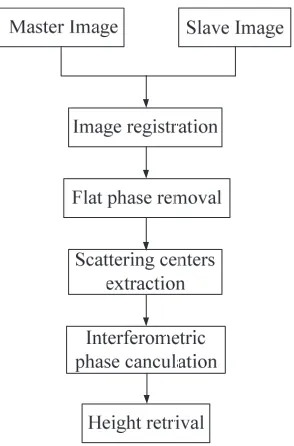
Without the consideration of the existence of phase glint, a flowchart of man-made target height retrieval used in [16] is shown as Fig. 2. Firstly, the flat phase is removed between the master image and slave image. Then, based on the scattering center model, the scattering centers are extracted from the master and slave images. Next, the interferometric phases of corresponding scatterer couples are obtained. In the man-made target height retrieval, the imaged scene is usually very small, and the maximum unambiguity height is much higher than the target height for most interferometric system configurations, implying that the target height can be directly estimated from the extracted interferometric phases. Finally, the target height is retrieved from the extracted interferometric phases as in Eq. (24). It should be pointed out that the retrieved height is a relative height. According to Section 3.1, if the extracted scatterer couples include those caused by phase glint, especially in the case that the interferometric phase exceeds the span decided by the elementary scatterers, the retrieved height will deviate greatly from the real one.
4. EXPERIMENTAL EXAMPLES
Table 1. Parameters of InSAR system.
System Parameter Value
Carrier frequency/GHz 10
Height of airplane/m 8000
Velocity of airplane/(m/s) 125
Looking angle/(◦) 45
Range resolution/m 1
Azimuth resolution/m 1
parameters of InSAR system in Sections 4.1 and 4.2 are listed in Table 1. In order to demonstrate the impact of phase glint on man-made target height retrieval, real data experiment is presented in Section 4.3.
4.1. Validation of Distribution of Interferometric Phase
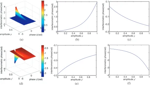
In simulation I, scatterers A and B are located at (0,8000,0) m and (0,8010,10) m, respectively, so it can be obtained that ΔϕA= 0.037 rad, ΔϕB=−0.4866 rad and ΔϕBA=−π6 ∈[−2π,0]. The span decided by the interferometric phases of the elementary scatterers is [−0.4866,0.037] rad. The distribution of ΔϕC when 0 ≤ ρ ≤ 1 is shown in Fig. 3(a), and the value range is [−0.2488,2.9168] rad, which is consistent with the theoretical value [ΔϕA+Δϕ2BA,ΔϕA+Δϕ2BA +π]. Fig. 3(b) and Fig. 3(c) represent the maximal and minimum value curves which are defined in Section 3.1, respectively. One can see that the maximal e and minimum value curves are the monotone increasing function and monotone decreasing function of ρ, respectively. The distribution of ΔϕC when ρ ≥1 is shown in Fig. 3(d), and the value range is [−3.3664,−0.2448] rad. From Fig. 3(e) and Fig. 3(f), it can be seen that the maximal value of ΔϕC is−0.2448 rad, and the minimum value is−3.3664 rad. Form Fig. 3(a) and Fig. 3(d), one can conclude that the value interval of ΔϕC is [−3.3664,2.9168] rad which obviously exceeds the span decided by interferometric phases of the elementary scatterers, and the dynamic range of ΔϕC is 2π, which are consistent with the theoretical value as shown in Eq. (19).
In simulation II, the coordinates of scatterer A are (0,8000,89.5) m, and the coordinates of scatterer
0 0.2 0.4 0.6 0.8 1 0
0.5 1 1.5 2 2.5 3
amplitude ρ
in
te
rf
e
ro
m
etr
ic
phas
e(
rad)
0 0.2 0.4 0.6 0.8 1 -0.3
-0.2 -0.1 0 0.1
amplitude ρ
in
te
rf
er
omet
ri
c
p
has
e(
rad)
0 0.2 0.4 0.6 0.8 1 -0.5
-0.4 -0.3 -0.2 -0.1
amplitude ρ '
in
te
rf
e
ro
m
et
ri
c
ph
as
e
(r
a
d)
0 0.2 0.4 0.6 0.8 1 -4
-3 -2 -1 0
amplitude ρ '
in
te
rf
e
ro
m
et
ri
c
ph
as
e(
ra
d)
(a) (b) (c)
(d) (e) (f)
Figure 3. Distribution of interferometric phase of simulation I. (a) Interferometric phase versusρandφ
(0≤ρ≤1). (b) The maximal value curve of interferometric phase versusρ (0≤ρ≤1,φ= 0.299 rad). (c) The minimum value curve of interferometric phase versus ρ (0 ≤ ρ ≤ 1, φ = −2.8426 rad). (d) Interferometric phase versus ρ and φ (ρ ≥ 1). (e) The maximal value curve of interferometric phase versus ρ (ρ ≥ 1, φ = 2.8426 rad). (f) The minimum value curve of interferometric phase versus ρ
(ρ≥1,φ =−0.299 rad).
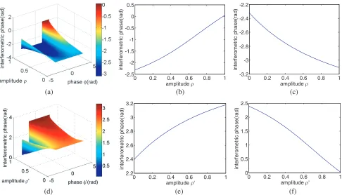
B are (0,7910.5,0) m, which means ΔϕA=−2.319 rad, ΔϕB = 2.3935 rad and ΔϕBA = 1.5π ∈[0,2π]. From Fig. 4, one can conclude that the value range of ΔϕC is [−3.3664,2.9168] rad, and the dynamic range of ΔϕC is 2π, which are consistent with the theoretical value as shown in Eq. (18).
4.2. Classical InSAR Image Processing Results
In this part, two simulation experiments of airborne InSAR are presented to analyze the impact of phase glint on classical InSAR image process. Both simulation scenarios share the same terrain, which is a flat plane with an area 400 m×400 m in both ground range direction and azimuth direction. Two group scatterers are set in both simulation experiments, and the coordinates are the same as in Section 4.1. The parametersρ andφof each simulation are shown in Table 2. In order to minimize the influence of the terrain to the interferometric phase of phase glint, the signal power to clutter power ratio (SCR) is set as 5 dB. Then, the classical image processing is applied to each simulation. The image results are shown as in Fig. 5 and Fig. 6, and the comparisons of the theoretical values and estimated values are shown in Table 2.
0 0.2 0.4 0.6 0.8 1 -2.5
-2 -1.5 -1 -0.5 0 0.5
amplitude ρ
in
te
rf
e
ro
m
etr
ic
phas
e(
rad)
0 0.2 0.4 0.6 0.8 1 -3.2
-3 -2.8 -2.6 -2.4 -2.2
amplitude ρ
in
ter
fer
ometr
ic
p
has
e(
rad)
0 0.2 0.4 0.6 0.8 1 2.2
2.4 2.6 2.8 3 3.2
amplitude ρ'
in
te
rf
e
ro
m
et
ri
c
ph
as
e
(r
a
d)
0 0.2 0.4 0.6 0.8 1 0
0.5 1 1.5 2 2.5
amplitude ρ'
in
te
rf
e
ro
m
et
ri
c
ph
as
e(
ra
d)
(a) (b) (c)
(d) (e) (f)
Figure 4. Distribution of interferometric phase of simulation II. (a) Interferometric phase versusρand
φ(0≤ρ≤1). (b) The maximal value curve of interferometric phase versusρ(0≤ρ≤1,φ= 2.3562 rad). (c) The minimum value curve of interferometric phase versus ρ (0 ≤ ρ ≤ 1, φ = −0.7853 rad). (d) Interferometric phase versus ρ and φ (ρ ≥ 1). (e) The maximal value curve of interferometric phase versus ρ (ρ ≥ 1, φ = 0.7853 rad). (f) The minimum value curve of interferometric phase versus ρ
(ρ≥1,φ =−2.3562 rad).
Table 2. Parameters setting and the comparison of the theoretical values and the estimated results of classical InSAR image processing.
ρ φ/(rad) ΔϕC/(rad) h/(m) Δ ˆϕC/(rad) h/ˆ (m)
Simulation III Scatterer group 1 0.7 −2.8426 −0.1783 4.1 −0.1747 4.04
Scatterer group 2 0.9 2.3562 −0.2156 49.4 −0.2117 49.3
Simulation IV Scatterer group 1 10/7 0.3 −1.5067 29.5 1.494 29.3
Scatterer group 2 0.5 −0.7856 −2.83 99.3 3.462 −20.3
Azimuth (m)
R
a
nge(
m
)
-200 -100 0 100 200 1.12
1.125
1.13
1.135
1.14
1.145 x 10⁴
Azimuth (m)
R
a
nge(
m
)
-200 0 200
1.12
1.125
1.13
1.135
1.14
1.145 x 10⁴
-3 -2 -1 0 1 2 3
Azimuth (m)
R
a
nge(m
)
-200 0 200
1.12
1.125
1.13
1.135
1.14
1.145 x 10⁴
-4 -2 0 2 4 6
(a) (b) (c)
(d) (e)
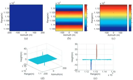
Figure 5. The InSAR image processing results of simulation III. (a) Master image. (b) Wrapped interferogram. (c) Unwrapped interferogram. (d) DEM. (e) Azimuth-height projection DEM.
Azimuth (m)
R
ange(m
)
-200 -100 0 100 200 1.12
1.125
1.13
1.135
1.14
1.145 x 10⁴
Azimuth (m)
R
a
nge(m
)
-100 0 100 1.12
1.125
1.13
1.135
1.14
1.145 x 10⁴
-3 -2 -1 0 1 2 3
Azimuth (m)
R
ange(m
)
-100 0 100 1.12
1.125
1.13
1.135
1.14
1.145 x 10⁴
-4 -2 0 2 4 6
(a) (b) (c)
(d) (e)
retrieval height is quite different from the real height of any elementary scatterer. In this case, the interferometric phase of phase glint exceeds the phase interval decided by the elementary scatterers, which will lead to serious height estimated error.
In sum, the interferometric phase of phase glint varies with the CSCR of elementary scatterers, and the retrieved height from the interferometric phase cannot reflect the real height of any elementary scatterer. When the interferometric phase exceeds the span decided by the interferometric phases of the elementary scatterers, it will produce serious height estimation error in classical InSAR image processing.
4.3. Man-Made Target Height Retrieval Results
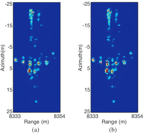
To demonstrate the impact of phase glint on man-made height retrieval, we apply the method presented in Section 3.3 to real data provided by East China Research Institute of Electronic Engineering. The data are acquired with carrier frequency of 9.6 GHz in single pass bistatic mode over Lingshui County of China. The spatial resolutions in the slant range and azimuth direction are both 0.3 m. The interferometric baseline is about 1.22 m with its orientation angle ε = 15.6◦. Considering that radar looking angle for the middle scene is about θ ≈50.3◦ (R0 ≈ 8.3 km, and H ≈5.3 km), we obtain the perpendicular baseline B⊥ = 1 m. The maximum unambiguity height is huamp = 198 m. For airplane target height retrieval, the unambiguity height is sufficient. We choose a slice of the real data, which corresponds to an airplane parked on the aerodrome. The real height of the airplane is about 11 m. Fig. 7 presents the SAR images of the airplane.
Range (m)
Azi
mu
th(m)
8333 8354
-25
-15
-5
5
15
25
Range (m)
Azi
mu
th(m)
8333 8354
-25
-15
-5
5
15
25
(a) (b)
Figure 7. SAR images of an airplane. (a) Master image. (b) Slave image.
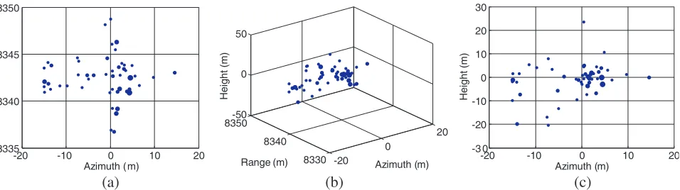
-20 -10 0 10 20 8335
8340 8345 8350
Range (
m
)
Azimuth (m) -20
0
20
8330 8340 8350-50
0 50
Azimuth (m) Range (m)
Height
(m)
-20 -10 0 10 20 -3 0
-20 -10 0 10 20 30
Height
(m)
Azimuth (m)
(a) (b) (c)
Figure 8. 3D reconstruction results for the airplane. (a) Range-azimuth projection map. (b) 3D representation of the scatterers. (c) Azimuth-height projection map.
5. CONCLUSION
In this paper, we investigate the phase glint problem caused by multiple scatterer interference of a single pixel in single-pass InSAR system. Our mathematic analysis indicates that the observed interferometric phase of phase glint is a chaotic value and varies with the CSCR between the elementary scatterers, which cannot reflect the real height of any elementary scatterer and may produce serious height estimating error. Simulation and real data experiment results verify the theoretical analysis. Our analysis and experimental results suggest that for height retrieval especially for man-made target, extra care is needed to account for the effects of phase glint caused by multiple scatterer interference.
Moreover, for the specialty of creating a chaotic interferometric in InSAR image processing, the phase glint can be utilized to develop three-dimension deceptive scene generation method against InSAR.
APPENDIX A.
This appendix will derive Equation (9). The first derivative off(ρ, φ) which is shown as in Eq. (8) with respect to φcan be expressed as
df(ρ, φ)
dφ =
ρ−ρ3(cos (φ+ ΔϕBA)−cosφ)
(1 +ρcos (φ+ ΔϕBA) +ρcosφ+ρcos ΔϕBA)2 (A1)
Let df(ρ,φ)dφ = 0, and the extreme points of f(ρ, φ) are derived as φ = −Δϕ2BA + ϕsA −ϕsB and
φ=π−Δϕ2BA +ϕsA−ϕsB.
Substitutingafor the denominator of the right of Eq. (A1), the second derivative of f(ρ, φ) with respect to ϕcan be written as
df2(ρ, φ)
dφ2 =
ρ−ρ3((sinφ−sin (φ+ ΔϕBA))a−(cos (φ+ ΔϕBA)−cosφ)a)
a2 (A2)
where a represents the derivative of a with respect to φ. When φ = −ΔϕBA
2 + ϕsA − ϕsB or
φ=π−Δϕ2BA +ϕsA−ϕsB, one can obtain that
df2(ρ, φ)
dφ2 =
⎧ ⎪ ⎪ ⎨ ⎪ ⎪ ⎩
−2ρ−ρ3sin (ΔϕBA/2)
a φ=−
ΔϕBA
2 +ϕsA−ϕsB 2ρ−ρ3sin (ΔϕBA/2)
a φ=π−
ΔϕBA
2 +ϕsA−ϕsB
(A3)
APPENDIX B.
Settingx= 1+ρρsin(Δϕcos(ΔϕBA/2)
BA/2)andy =
ρsin(ΔϕBA/2)
1−ρcos(ΔϕBA/2), and substituting into ΔϕC max(ρ)andΔϕC min(ρ)
which are expressed by Eqs. (14) and (15), respectively, the derivatives of ΔϕC max(ρ) and ΔϕC min(ρ) with respect toρ can be expressed as
ΔϕC max(ρ) =
⎧ ⎪ ⎪ ⎪ ⎨ ⎪ ⎪ ⎪ ⎩
2 sin (ΔϕBA/2)
(1 +x2) (1 +ρcos (ΔϕBA/2))2 ΔϕBA∈(0,2π) + 4kπ
− 2 sin (ΔϕBA/2)
(1 +y2) (1−ρcos (Δϕ
BA/2))2
ΔϕBA∈(−2π,0) + 4kπ
(B1)
ΔϕCmin(ρ) =
⎧ ⎪ ⎪ ⎪ ⎨ ⎪ ⎪ ⎪ ⎩
− 2 sin (ΔϕBA/2)
(1 +y2) (1−ρcos (ΔϕBA/2))2 ΔϕBA∈(0,2π) + 4kπ 2 sin (ΔϕBA/2)
(1 +x2) (1 +ρcos (Δϕ
BA/2))2
ΔϕBA∈(−2π,0) + 4kπ
(B2)
From Eqs. (B1) and (B2), it can be seen that ΔϕC max(ρ)≥0 and ΔϕC min(ρ)≤0 for arbitrary ΔϕBA, i.e., ΔϕC max(ρ) is monotone increasing function while ΔϕC min(ρ) is monotone decreasing function of ρ. So, ΔϕC max(ρ) and ΔϕC min(ρ) have maximal value and minimum value, respectively, when
ρ = 1, which are also the maximal and minimum values of ΔϕC. Moreover, it can be concluded that min(ΔϕC max(ρ)) = max(ΔϕC min(ρ)) = ΔϕA. In summary, the value range of ΔϕC(ρ, ϕ) is equal to the union of the range of ΔϕC max(ρ) and ΔϕC min(ρ). So, one can obtain
max (ΔϕC) = ΔϕC max(1) =
⎧ ⎪ ⎪ ⎪ ⎨ ⎪ ⎪ ⎪ ⎩
ΔϕA+ 2 tan−1
sin (ΔϕBA/2) 1 + cos (ΔϕBA/2)
ΔϕBA∈(0,2π) + 4kπ
ΔϕA−2 tan−1
sin (ΔϕBA/2) 1−cos (ΔϕBA/2)
ΔϕBA∈(−2π,0) + 4kπ (B3)
min (ΔϕC) = ΔϕCmin(1) =
⎧ ⎪ ⎪ ⎪ ⎨ ⎪ ⎪ ⎪ ⎩
ΔϕA−2 tan−1
sin (ΔϕBA/2) 1−cos (ΔϕBA/2)
ΔϕBA∈(0,2π) + 4kπ
ΔϕA+ 2 tan−1
sin (ΔϕBA/2) 1 + cos (ΔϕBA/2)
ΔϕBA∈ (−2π,0) + 4kπ (B4)
For a given ΔϕBA, there is always a ΔϕBA∈[−2π,2π] satisfying ΔϕBA= ΔϕBA−4kπ. According to submultiple angle formula of trigonometric functions
tan−1
sin (ΔϕBA/2) 1−cos (ΔϕBA/2)
= ⎧ ⎪ ⎨ ⎪ ⎩ π 2− ΔϕBA
4 ΔϕBA∈(0,2π) + 4kπ
−π
2− ΔϕBA
4 ΔϕBA∈(−2π,0) + 4kπ
(B5)
tan−1
sin (ΔϕBA/2) 1+ cos (ΔϕBA/2)
= Δϕ
BA
4 (B6)
Then, it can be concluded that
ΔϕA−2 tan−1
sin (ΔϕBA/2) 1−cos (ΔϕBA/2)
= ⎧ ⎪ ⎨ ⎪ ⎩
ΔϕA+ ΔϕBA
2 −π ΔϕBA∈(0,2π) + 4kπ ΔϕA+
ΔϕBA
2 +π ΔϕBA∈(−2π,0) + 4kπ
(B7)
ΔϕA+ 2 tan−1
sin (ΔϕBA/2) 1 + cos (ΔϕBA/2)
= ΔϕA+ ΔϕBA
2 (B8)
So for the case of 0≤ρ≤1, we can conclude that
ΔϕC∈
[ΔϕA+ ΔϕBA/2−π,ΔϕA+ ΔϕBA/2], ΔϕBA∈(0,2π) + 4kπ [ΔϕA+ ΔϕBA/2,ΔϕA+ ΔϕBA /2 +π], ΔϕBA∈(−2π,0) + 4kπ
REFERENCES
1. Cumming, I. G. and F. K. Wong,Digital Processing of Synthetic Aperture Radar Data: Algorithm and Implementation, Artech House, Norwood, MA, 2005.
2. Henke, D., C. Magnard, M. Frioud, et al., “Moving-target tracking in single-channel wide-beam SAR,”IEEE Trans. on Geosci. Remote Sens., Vol. 50, No. 11, 4735–4747, 2012.
3. Mouche, A. A., F. Collard, B.Chapron, et al., “On the use of doppler shift for sea surface wind retrieval from SAR,”IEEE Trans. on Geosci. Remote Sens., Vol. 50, No. 7, 2901–2909, 2012. 4. Zhou, J. X., Z. G. Shi, X. Cheng, et al., “Automatic target recognition of SAR imagesbased on
global scattering center model,” IEEE Trans. on Geosci. Remote Sens., 3713–3729, 2011.
5. Papson, S. and R. M. Narayanan, “Classification via the shadow region in SAR imagery,” IEEE Trans. on Aerospace and Electronic Systems, Vol. 48, No. 2, 969–980, 2012.
6. Dabboor, M., M. J. Collins, V. Krrathanassi, et al., “An unsupervised classification approach for polarimetric SAR data based on the chernoff distance for complex wishart distribution,” IEEE Trans. Geosci. Remote Sens., Vol. 51, No. 7, 4200–4213, 2013.
7. Zhu, X. X. and R. Bamler, “Tomographic SAR inversion by L1-norm regularization — The Compressive Sensing Approach,” IEEE Trans. Geosci. Remote Sens., Vol. 48, No. 10, 3839–3846, 2010.
8. Xing, S. Q., Y. Z. Li, D. H. Dai, et al., “Three-dimensional reconstruction of man-made objects using polarimetric tomographic SAR,” IEEE Trans. Geosci. Remote Sens., Vol. 51, No. 6, 3694– 3705, 2013.
9. Rosen, P. A., S. Hensley, I. R. Joughin, et al., “Synthetic aperture radar interferometry,” Proc. IEEE, Vol. 88, No. 3, 333–382, 2000.
10. Berardino, P., G. Fornaro, R. Lanari, et al., “A new algorithm for surface deformation monitoring based on small baseline differential SAR interferograms,” IEEE Trans. Geosci. Remote Sens., Vol. 40, No. 11, 2375–2383, 2002.
11. Cloude, S. R. and K. P. Papathanassiou, “Polarimetric SAR interferometry,”IEEE Trans. Geosci. Remote Sens., Vol. 36, No. 5, 1551–1565, 1998.
12. Papathanassiou, K. P. and S. R. Cloude, “Single baseline polarimetric SAR interferometry,”IEEE Trans. Geosci. Remote Sens., Vol. 39, No. 11, 2352–2363, 2001.
13. Zhu, X. X. and R. Bamler, “Demonstration of super-resolution for tomographic SAR imaging in urban environment,”IEEE Trans. Geosci. Remote Sens., Vol. 50, No. 8, 3150–3157, 2012.
14. Austin, C. D. and R. L. Moses, “IFSAr processing for 3D target reconstruction,” Algorithms for Synthetic Aperture Radar Imagery XII, SPIE Defense and Security Symposium, Orlando, 2005. 15. Austin, C. D. and R. L. Moses, “Interferometric synthetic aperture radar detection and estimation
based 3D image reconstruction,” Algorithms for Synthetic Aperture Radar Imagery XIII, SPIE Defense and Security Symposium, Orlando, 2006.
16. Xing, S. Q., “Study on the 3D imaging of manmade target based on polarimetric radar,”
ChinaNational University of Defense Technology, 2013.
17. Pauciullo, A., D. Reale, A. D. Maio, et al., “Detection of double scatterers in SAR tomography,”
IEEE Trans. Geosci. Remote Sens., Vol. 50, No. 9, 3567–3586, 2012.
18. Lombardini, F. and M. Pardini, “Superresolution differential tomography: Experiments on identification of multiple scatterers in spaceborne SAR data,” IEEE Trans. Geosci. Remote Sens., Vol. 50, No. 4, 1117–1129, 2012.