Multiple-GPU-Based Frequency-Dependent Finite-Difference Time
Domain Formulation Using MATLAB Parallel Computing Toolbox
Wenyi Shao* and William McCollough
Abstract—A parallel frequency-dependent, finite-difference time domain method is used to simulate electromagnetic waves propagating in dispersive media. The method is accomplished by using a single-program-multiple-data mode and tested on up to eight NVidia Tesla GPUs. The speedup using different numbers of GPUs is compared and presented in tables and graphics. The results provide recommendations for partitioning data from a 3-D computational model to achieve the best GPU performance.
1. INTRODUCTION
The FD-FDTD method [1] provides a way to model electromagnetic problems in dispersive media. This approach requires to compute the electric displacement vector (or called D field) before updating the electric field, as such is more time-consuming and uses more memory than a regular FDTD (non-frequency-dependent) simulation. Parallel computing techniques allow for improved computational efficiency when treating large-scale computational problems, particularly when using GPU.
Modern GPUs are more efficient in processing data than general-purpose central processing unit (CPU) due to their parallel structures. However, the small memory of GPUs limits their ability to solve large-scale electromagnetic problems. As the cost of GPUs reduces, using multiple GPUs to accelerate computations becomes more attractive. Commercial software, such as Computer Simulation Technology Microwave Studio (CST MWS) [2], has integrated multi-GPU packages for solving electromagnetic problems. However, analysis of CST MWS models, including calculation of parameters for later simulation and meshing the models to ensure computation convergence, can be time-consuming and cost-prohibitive. Thus, there is a demand for researchers to develop the required software tools to solve particular electromagnetic problems. Due to the complexity of GPU programming, using multiple GPUs for FD-FDTD is still rare in scientific literature.
There are two major approaches to programming multi-GPU based parallel FD-FDTD: open computing language (OpenCL) [3, 4] and compute unified device architecture (CUDA) [5–8]. OpenCL is a framework and programming language that executes across heterogeneous platforms consisting of CPUs, GPUs, or other processors. OpenCL has been used to simulate electromagnetic waves interacting with plasma by GPUs in [9]. CUDA is a parallel computing platform and application programming interface (API) designed by NVidia [10], which is more widely used than OpenCL recently. Zunoubi and his colleagues, in 2011, presented the first message passing interface CUDA (MPI-CUDA) FDTD implementation in dispersive media using Open multi-processing (Open-MP) to synchronize the operation of GPUs and CPUs [5, 6]. A whole-body electromagnetic simulation over the frequency range 70 to 2000 MHz was performed. Different types of GPUs were used to compare their real computability. Researchers from Belgium used CUDA on up to four GPUs for a 3-D FDTD application with multi-pole dispersion for plasma [7, 8], and found an almost linear speedup with respect to the number of GPUs.
Received 17 July 2017, Accepted 14 September 2017, Scheduled 15 September 2017
* Corresponding author: Wenyi Shao ([email protected]).
In 2013, Zhou et al. developed a 3D-FDTD GPU-based software using CUDA for earthquake engineering and disaster management [11]. Since OpenCL and CUDA rely on an advanced language and require GPU memory pre-administration when performing data transfer between GPUs, developers must be familiar with GPU memory hierarchy, multiple-GPU address space (unified virtual address (UVA)) [12], and the advanced language to take advantage of parallel FD-FDTD with GPU. It might not be easy for electromagnetics researchers to quickly start multiple GPU parallel computing without these experiences.
MATLAB [13] is a computing environment and programming language with millions of users in industry and academia due to its ease of operation and accessibility of data. GPU computing has been supported in MATLAB since version R2010b, but not until version R2016a was released, was data passing across GPUs supported. The parallel computing toolbox V6.8 in R2016a and later versions (most recent parallel computing toolbox is V6.10 in MATLAB R2017a) allow running parallel FDTD on multiple GPUs within the MATLAB environment. The prime advantage using MATLAB parallel computing toolbox to process multiple GPU task is that programmer does not need to consider the length of data for passing between GPUs, but which is required by conventional CUDA-based multiple-GPU operation that data for transferring has to be pre-evaluated, and pre-allocated in terms of the size of blocks and grids on the target GPU memory. The method discussed in this paper takes advantage of standard MATLAB language to program parallel FD-FDTD on multiple GPUs. The presented method does not need any CUDA coding in MATLAB, or require writing C/C++ in a MATLAB executable (MEX) function to operate GPUs. It is not even necessary for the programmer to understand GPU’s memory hierarchy. Therefore, it allows researchers to perform a fast use of accelerated FDTD computation without any CUDA background or sophisticated C/C++ knowledge. And the entire program can be greatly reduced and simplified. Our method uses a SPMD mode and will be elaborated in Section 2 in this paper. In the third section, performance using different numbers of GPUs is presented. Conclusions and suggestions to fully use the capability of GPUs are made in the last section.
2. COMPUTATIONAL MODEL AND GPU-BASED FDTD METHOD
The human knee replica in our test is a computational model with dielectric properties defined by Gabriel’s 4-pole-Cole-Cole equation [14] and based on anatomical data from Christ et al. in 2010 [15]. For simpler FD-FDTD programming, we map the 4-pole-Cole-Cole data to a one-pole Debye model as in Equation (1).
˜
ε(ω) =ε∞+εs−ε∞ 1 +jωτ −j
σs
ωε0
(1)
where ε∞ is the permittivity value at infinite high frequency, εs the static permittivity, τ the characteristic relaxation time, σs the static conductivity, and ε0 the permittivity in a vacuum. The
constructed Debye model and Cole-Cole model are in good agreement within a frequency range from 1 to 10 GHz for all tissues. Equation (1) is inserted into the constitutive equation D= ˜ε(ω)E to update the E field by an electric displacement field D, and then by the E field the next half-step H field is computed. Thus, the sequence for field updating in FD-FDTD is En → Hn+12 → Dn+1 → En+1. To update theE field, the past two steps of theDfield and the Efield are required, so memory limitation becomes problematic when a small number of GPUs are available.
In this paper, tests are conducted on up to eight NVidia Tesla GPUs mounted on a 24-core server. Each GPU has 6 GB of available memory. The following describes our parallel FD-FDTD program while using eight GPUs in more detail. Our program starts by creating a MATLAB parallel pool containing eight MATLAB workers (MATLAB names each node as a worker), each controlling a GPU. To parallelize FD-FDTD, we distribute the model parameters (EP s=εs,EP inf =ε∞,TAO=τ, and SIGMA= σs) to the GPUs. This is accomplished by creating a SPMD statement using the following MATLAB codes
spmd (n)
.. .
ep sG=gpuArray(getLocalPart(ep s)); ep infG=gpuArray(getLocalPart(ep inf)); taoG=gpuArray(getLocalPart(tao)); sigmaG=gpuArray(getLocalPart(sigma));
.. .
This is the first of two SPMD statements in the entire program. Here, nis the number of GPUs used (in this case n = 8), and ep sG, ep infG, taoG, and sigmaG are GPU-data forms of the four parameters. The parameter codistributor 1d (3) denotes that the computational object model will be split along the third dimension (in our case, Z axis in Figure 1). Data are distributed in CPU memory and then passed to corresponding GPUs with the gpuArray ( )function. If gpuArray ( ) were dismissed, multi-CPU-core parallelization would occur instead. In some existing examples, each SPMD statement must start with a gpuDevice (labindex) instruction to call a corresponding GPU device. However, our tests have shown that this is not necessary.
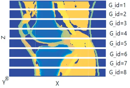
Figure 1. A Z-X cross plane of the knee model. The 3-D knee model is partitioned along the Z direction and evenly allocated to eight GPUs.
Figure 1 shows the computed dielectric constant at 4 GHz in aZ-X cross plane of the knee model saved in each GPU. The dimension of the entire knee model is Numx= 320, Numy= 320, Numz= 360 creating about 37 Megavoxels. The cells are 0.5 mm in each dimension (X, Y, and Z). Additionally, all field variables (D, E, and H fields) are initialized in this SPMD statement. For example, the
z-component of theD field is initialized by the following:
Dz=zeros (Numx, Numy, Numz/numlabs, ‘gpuArray’);
where numlabs denotes the number of GPUs. Since data are evenly partitioned along the Z axis, the length in the Z direction for each field variable is Numz/numlabs in every GPU, which in this case is equal to 45. The interfaces (2-D matrix to be passed) between GPUs are matrices of size 320×320.
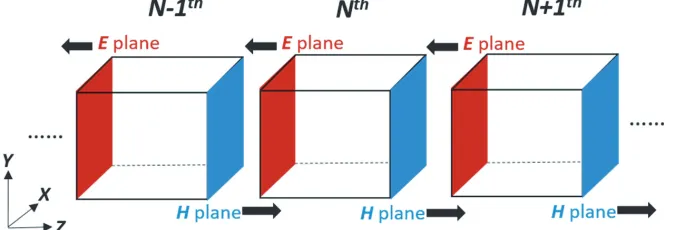
Figure 2 shows the data exchange ofE andH planes between GPUs. TheEx andEy fields on the interfaces are delivered exclusively from the right GPUs to the left GPUs. TheHx andHy fields on the interfaces are delivered exclusively from the left GPUs to the right GPUs. TheDfields do not exchange between GPUs. This data-exchange approach was applied in [3] and [8], and in the multi-CPU-core FDTD [16]. In MATLAB, this exchange can be defined by a data movement direction within the first SPMD statement. The following MATLAB code is an example to specify acquiring data from a lower indexed GPU, and sending data to the next higher indexed GPU for theH field:
if labindex<numlabs; labTo=labindex+1; else
if labindex>1; labFrom=labindex-1; else
labFrom=[ ]; end
where labindexis a GPU index. Similar codes can be used to specify the data movement direction for theE field.
Figure 2. Interface (between GPUs) data exchanges between GPUs: E planes (red) are delivered from theN+ 1th GPU to theNth GPU, from the Nth GPU to theN−1th GPU. . . in order to update the
Hfield in the blue planes in theNth,N −1th. . . GPU; Then in the next half time step,Hplanes (blue) are delivered from the N−1th GPU to theNth GPU, from the Nth GPU to the N + 1th GPU. . . in order to update the E field in red planes in theNth, N + 1th. . . GPU.
In the second SPMD statement in the program, standard FD-FDTD equations were used to update theE-field,D-field, and H-field data, and use the MATLABlab Send Receivefunction to transfer data. The Hy and Hx fields on the interfaces are transferred using the following codes:
Hyp=labSendReceive(labTo,labFrom,Hy(:,:,Numz/numlabs)); Hxp=labSendReceive(labTo,labFrom,Hx(:,:,Numz/numlabs));
whereHy(:,:,Numz/numlabs)and Hx(:,:,Numz/numlabs)are theHy and Hx fields on the interfaces, and labTo and labFrom have been defined in the first SPMD statement. Since the Hy and Hx fields were initialized as GPU data in the first SPMD statement, the labSendReceive function will transfer data among GPUs. A similar operation can be made to pass the Ey and Ex field data. If all the field variables were created and distributed in CPU memory only, labSendReceive would transfer data only between CPUs, which is a multi-CPU-based parallelization mode. It is ambiguous as to how the data passed will be physically stored in the target GPU. It is not necessary to specify the address or allocate memory in the target GPU for the transferred data, as required in CUDA. In addition, it is important to note that thelabSendReceivefunction only allows for passing data between GPUs in MATLAB 2016a parallel computing toolbox V6.8 and later versions. Using any earlier version causes an error.
To validate the MATLAB multi-GPU FD-FDTD program, we placed an excitation, polarized in the
Y direction in front of the knee in the G id= 4 GPU’s computational area in Figure 1 and placed two probes behind the knee (G id= 1 and G id= 8 GPU’s computational area in Figure 1, respectively). Liao et al.’s 2nd order boundary condition [17] was used to truncate the computational area. The simulation took 673 seconds to complete 5,000 time steps using eight GPUs. The same computational model and simulation with FD-FDTD on a CPU without any parallelization took 18 hours using an Intel core i7 CPU (2.70 GHz, with 32-GB memory). The time-domain waveforms obtained at two probes, in both the eight GPU and CPU FD-FDTD simulation, were found to be essentially the same, as shown in Figure 3.
3. SPEEDUP USING MULTIPLE GPUS
(a) (b)
Figure 3. Comparison of the time-domainE-field signal obtained by eight GPU parallelization and a single CPU at (a) probe 1 and (b) probe 2.
with FD-FDTD on other computational models is also evaluated. All results are presented using an average of three runs in each case.
We approached the same electromagnetic problem described in Section 2 using two, four, and eight GPUs, respectively, while using the same server in each case. We were unable to run this computation on a single GPU because of our GPU’s memory limitation. Speedup using eight GPUs versus four GPUs, and four GPUs versus two GPUs, is compared in Table 1. Table 1 shows that the speedup is almost linear with respect to the number of GPUs.
Table 1. The speedup with three different number of GPUs using the 320×320×360 model.
Number of GPU N = Time to complete 5000 steps (seconds) Speedup versus N/2 GPUs
2 2171
-4 1186 1.831
8 673 1.762
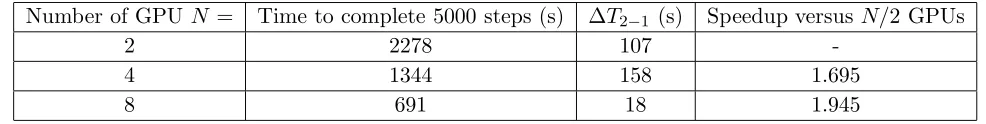
In [5], Mega voxels times the number of time steps divided by the required simulation time was used to reveal the computing ability of a GPU cluster. This method is controversial as it ignores the impact of data passing between GPUs. The knee model is repositioned, so the longest side becomes the first dimension, i.e., 360×320×320. To achieve the best computational performance, allocation is always along the third dimension. Thus, data sent between GPUs are matrices of size 360×320, which require longer data passing time. We used two, four, and eight GPUs, respectively, to simulate the rearranged knee model, using the same server in each case. Table 2 presents the completion time of simulations by two, four, and eight GPUs. The entire execution time is longer than that in Table 1 for all three cases. The extra time needed for the 360×320×320 model compared to the 320×320×360 model is denoted by ΔT2−1, presumably due to additional data passing.
The results in Table 1 and Table 2 might indicate that a 3-D model with a smaller interface will require less total execution time (assuming total number of voxels remain the same), as the data
Table 2. The speedup with three different numbers of GPUs using the 360×320×320 model.
Number of GPU N = Time to complete 5000 steps (s) ΔT2−1 (s) Speedup versusN/2 GPUs
2 2278 107
-4 1344 158 1.695
passing is minimal while distribution is along the longest side, but this is not always the case. In a single computational unit (such as one GPU), MATLAB/C executes loops faster in lower dimensions than in higher dimensions. For example, if a single GPU is given two sub-data blocks for computation (320× 320 ×45 and 360×320 ×40), their total voxels are identical, but the latter requires less computational time because the first dimension is larger, and the third dimension is smaller. However, when taken in the context of the entire computation across multiple GPUs, the latter requires greater time because of passing larger matrices between GPUs. Therefore, there will be a tradeoff between computations and data communications between GPUs.
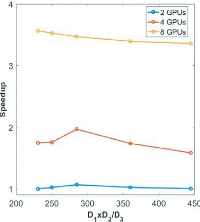
To check our hypothesis, we tested five 3-D data blocks in FD-FDTD: 320×288×400, 320×300×384, 320×320×360, 360×320×320, and 400×320×288. These data blocks are obtained by expanding or reducing the margins in the above knee model. The number of voxels in all models is the same. D1,
D2, and D3 represent the length in each dimension. So D1×D2, representing the data quantity to be
passed, increases from the first model to the last model; D3 decreases from the first model to the last
model, corresponding to a D1×D2/D3 value increasing from the first model to the last model (as in
from 230, 250, 284, 360, to 444). The speed to complete 5,000 time steps for each of the five data blocks using two, four, and eight GPUs is shown in Figure 4. The vertical axis represents the speedup, and the horizontal axis represents the variation of D1×D2/D3. The slowest case when using two GPUs is
in the 320×288×400 model, where the speed is denoted as 1 on the “Speedup” axis. All other cases express speed based on a ratio to the slowest case. The 320×320×360 model balances the computation and data passing best when two or four GPUs are used as it corresponds to the maximum point on the curve. The fastest case when using eight GPUs is in the 320×288 ×400 model. The curve of eight GPUs does not appear as convex as the two and four GPUs, but it does not mean an optimum never exists. A convex curve for eight GPUs can be expected when a larger model containing more voxels is processed. When a small number of GPUs is used, each GPU is correspondingly allocated a large computational task, so the computational efficiency of the GPU is more important than data communications between GPUs. In contrast, when many GPUs are used, each GPU is correspondingly allocated a small computational task, so data communication between GPUs becomes a consideration. In addition, Figure 4 indicates appropriate selection of the third dimension for distribution in a 3-D model. When four GPUs are used, each GPU is allocated 9.25 Mega voxels in each of the five data blocks. So, regarding the NVidia Tesla GPU in our test, when a GPU is assigned a computational task larger than 9.25 Mega voxels in parallel FD-FDTD computation, the tradeoff between computation and
communication needs to be considered. TheD1×D2/D3 value presented in Figure 4 indicates optimal
selection of the third dimension. When a GPU is assigned significantly fewer than 9.25 Mega voxels, the longest side of the model should be selected for distribution between GPUs.
4. CONCLUSIONS
We presented a multi-GPU based frequency-dependent FDTD method using MATLAB for large-scale dispersive electromagnetic problems using NVidia Tesla GPU cards. In the presented method, there is no need to administer GPU memory when passing data between GPUs. We described how the computational model’s size affects the computational efficiency which, in turn, advises researchers to create appropriately sized computational models and to determine the model partition strategy (per the number of GPUs). When there are many GPUs, the longest side of the model should be considered as the third dimension for data distribution to minimize data passing. The second longest side should be selected as the first dimension to achieve a fast-computational speed. When the number of available GPUs is small, more consideration should be given to the computational efficiency of each GPU. The value of D1×D2/D3 suggests how a 3-D model should be partitioned.
REFERENCES
1. Luebbers, R., F. P. Hunsberger, K. S. Kunz, R. B. Standler, and M. Schneider, “A frequency-dependent finite-difference time-domain formulation for dispersive materials,” IEEE Trans. Electromagn. Compat., Vol. 32, 222–227, 1990.
2. Computer Simulation Technology Microwave Studio, https://www.cst.com/products/cstmws. 3. Stefanski, T. P., N. Chavannes, and N. Kuster, “Multi-GPU accelerated finite-difference
time-domain solver in open computing language,” PIERS Online, Vol. 7, 71–74, 2011.
4. Stefanski, T. P., N. Chavannes, and N. Kuster, “Parallelization of the FDTD method based on the open computing language and the message passing interface,” Microwave Opt. Technol. Lett., Vol. 54, 785–789, 2012.
5. Zunoubi, M. R., J. Payne, and M. Knight, “FDTD multi-GPU implementation of Maxwell’s equations in dispersive media,” Optical Interactions with Tissue and Cells XXII, Vol. 7897, 1– 6, 2011.
6. Zunoubi, M. R., J. Payne, and W. P. Roach, “CUDA-MPI-FDTD implementation of Maxwell’s equations in general dispersive media,”Optical Interactions with Tissue and Cells XXIII, Vol. 8221, 1–6, 2012.
7. Wahl, P., C. Debaes, J. V. Erps, N. Vermeulen, D. A. B. Miller, and H. Thienpont, “B-Calm: An open-source multi-GPU-based 3D-FDTD with multi-pole disperion for plasmonics,” Progress In Electromagnetics Research, Vol. 138, 467–478, 2013.
8. Baumeister, P. F., T. Hater, J. Kraus, D. Pleiter, and P. Wahl, “A performance model for GPU-accelerated FDTD applications,” 2015 IEEE 22nd International Conference on High Performance Computing, 185–192, 2015.
9. Cannon, P. D. and F. Honary, “A GPU-accelerated finite-difference time-domain scheme for electromagnetic wave interaction with plasma,” IEEE Trans. Antennas Propag., Vol. 63, 3042– 3054, 2015.
10. NVIDIA official, websitehttp://www.nvidia.com.
11. Zhou, J., Y. Cui, E. Poyraz, D. J. Choi, and C. C. Guest, “Multi-GPU implementation of a 3D finite-difference time domain earthquake code on heterogenous supercomputers,”International Conference on Computational Science, Vol. 18, 1255–1264, 2013.
12. NVIDIA CUDA C Programming Guide, Chapter 3.2, 19–58, available in http://docs.nvidia.com/ cuda/cuda-c-programming-guide/index.html#axzz4rGDZXQXi.
14. Gabriel, S., R. W. Lau, and C. Gabriel, “The dielectric properties of biological tissues: III. Parametric models for the dielectric spectrum of tissues,” Phys. Med. Bio., Vol. 41, 2271–2293, 1996.
15. Christ, A., W. Kainz, E. G. Hahn, K. Honegger, M. Zefferer, E. Neufeld, W. Rascher, R. Janka, W. Bautz, J. Chen, B. K. P. Schmitt, H.-P. Hollenbach, J. Shen, M. Oberle, D. Szczerba, A. Kam, J. W. Guag, and N. Kuster, “The virtual family-development of surface-based anatomical models of two adults and two children for dosimetric simulations,” Phys. Med. Biol., Vol. 55, 23–38, 2010. 16. Hanawa, T., M. Kurosawa, and S. Ikuno, “Investigation on 3-D implicit FDTD method for parallel
processing,” IEEE Trans. Magnetics, Vol. 41, 1696–1699, 2005.