Pressure evaluation during dam break using weakly compressible SPH

(1)

Pressure evaluation during dam break using weakly

com-pressible SPH

PetrJanˇcík1,∗_and _Tomáš_Hyhlík1,∗∗

1_{Department of Fluid Dynamics and Thermodynamics, Faculty of Mechanical Engineering, Czech Technical University in Prague,}

Technická 4, 166 00 Praha 6, Czech Republic

Abstract.This paper presents a solution of a dam break problem in two dimensions obtained with smoothed particle hydrodynamics (SPH) method. The main focus is on pressure evaluation during the impact on the wall. The used numerical method and the way of pressure evaluation are described in detail. The numerical results of the kinematics and dynamics of the flow are compared with experimental data from the literature. The abilities and limitations of the used methods are discussed.

1 Introduction

A Dam-break problem is a relatively widely studied free-surface problem. In its simplest configuration, a liquid col-umn collapses in a gravity field, forming a surge on a flat dry bed of a tank. The surge then impacts a vertical wall of the tank, shaping a vertical jet along the wall and a rolling wave afterwards. The relative simplicity of the problem makes it suitable for both experimental and numerical in-vestigation.

The experimental works dealt mainly with kinematics and dynamics of the flow. Martin et al. investigated the position of the surge front and the height of the column as a function of time [1]. Lobovský et al. focussed primar-ily on pressure loads on the vertical wall during the surge impact; pressure was measured in various heights above the bottom of the tank, and the results were statistically evaluated [2].

Works dealing with a numerical solution of the dam break problem were often combined with an experiment, which proved the numerical method to be capable of sim-ulating free-surface flows. Such works are for example Koshizuka and Oka (moving particle semi-implicit) [3], Cruchaga et al. (finite element method) [4], and Hu and Sueyoshi (constrained interpolation profile and moving particle semi-implicit) [5]. These works deal only with the kinematics of the flow.

Some works presenting numerical solution of free-surface flows using SPH have also been published. These which dealt with dynamics of the flow are for example Co-lagrossi and Landrini [6], Ferrari et al. [7], and Laigle and Labbe [8]. All these authors compared their results with experimental data published by Zhou et al. [9].

The aim of this paper is to present a method of pres-sure evaluation in SPH and compare the obtained results

∗_{e-mail: petr.jancik@fs.cvut.cz} ∗∗_{e-mail: tomas.hyhlik@fs.cvut.cz}

with experimental data published in [2]. Two main issues to address in order to reach this goal are a correct formula-tion of wall boundary condiformula-tion, and pressure oscillaformula-tions occurring in weakly compressible SPH solution. The basic kinematics of the flow is compared with the experiment as well to validate the method.

2 Computational method

SPH is a mesh-free particle method. Its Lagrangian na-ture makes it suitable for free-surface and multi-phase flow problems because interfaces are tracked naturally. The governing equations of fluid motion, continuity and mo-mentum equation, in the Lagrangian framework are

D̺

Dt =−̺∇v, (1)

Dv Dt =−

1

̺∇p+f, (2)

wheret,̺,v,p, andfdenote time, density, velocity, pres-sure, and external body force. Fluid is modelled as invis-cid.

Since the fluid is considered to be compressible, an equation of state is needed to close the system of equa-tions. It is common in weakly compressible SPH that an artificial equation of state is employed. In this case a sim-ple equation

p=c2(̺−̺0) (3)

(2)

would become time expensive [10]. Note that the equation of state is not a function of temperature or internal energy thus energy equation does not have to be solved.

Using SPH techniques, partial differential equations (1) and (2) are spatially discretised and transformed into the following ordinary differential equations:

D̺i Dt =̺i

X

j mj

̺j

(vi−vj)· ∇Wi j+Di, (4)

Dvi Dt =−

X j mj pi ̺2 i

+ pj

̺2 j

+ Πi j

!

∇Wi j+fi. (5)

Indices i and j denote particles, m is mass, and Wi j is so called smoothing function. There are more smoothing functions. In this work, the truncated Gaussian smoothing function was employed, which can be written as

W(R,h)=

                  

π−d

2h−de−R2 ifR<3

0 ifR≥3

, (6)

where h is so-called smoothing length d is number of spatial dimensions, and non-dimensional particle distance R =|xj−xi|/h, wherexdenotes a vector of spatial coor-dinates. The truncation of the function does not affect the solution, but it has a significant effect on computational performance because the number of interacting particles is reduced.

There is an additional diffusive term in discretised con-tinuity equation (4). In more detail, it can be written as

Di=2δhc

X

j

(̺j−̺i)

(xj−xi)· ∇Wi j (xi−xj)·(xi−xj)

, (7)

whereδ is a coefficient of diffusion. This term reduces pressure oscillations in the solution [11].

Another additional termΠi jin the discretised momen-tum equation (5) is an artificial viscosity term. It serves for stabilisation of the numerical solution, and it can be written as

Πi j =max

h

−αci jhi j

̺i j

(vi−vj)·(xi−xj) (xi−xj)·(xi−xj)+εh2_{i j}

,0i, (8)

whereαis a tuning parameter and term with ε prevents singularity. All variables with both indicesiand jdenote a mean value taken from particlesiand j.

Fluid is considered to be inviscid, so wall boundary condition is modelled as a free-slip. Walls are made of three layers of so-called dummy particles, which take part in summations in equations (4) and (5). Using this ap-proach, particles near walls are uniformly surrounded by neighbouring particles and field variables can be evaluated correctly. The pressure of a dummy particle is determined by the formula

pw=

P

fpfWwf +Pfff ·(xw−xf)̺fWwf

P

fWwf

, (9)

where indiceswandf denote wall and fluid particle [12]. Density is then obtained from the equation of state (3). Dummy particle velocities are set to zero.

To further refine the obtained pressure field, density reinitialisation is conducted. New density values are ob-tained using the formula

̺i=

P

jmjWi j

P

j mj ̺jWi j

. (10)

This reinitialization is performed every 20 time steps. It is similar to what used Colagrossi and Landrini [6] but with simpler zero-order Shepard function [13].

Pressure values at certain locations are evaluated using virtual sensors. These sensors obtain values of pressure from fluid particles in the vicinity using the formula

pS =

P

jpjWS j

P

jWS j

, (11)

where indexS denotes sensor.

The size of the sensor influence domain is dependent on the smoothing lengthhof a smoothing functionW. Too small value of the smoothing length leads to fewer inter-acting influencing particles and noisy output. On the other hand, if the smoothing length is too great, distant parti-cles are taken into account and the output is not correct. A good choice of smoothing length appears to be the same value as the one used in the simulation. For this choice, the sensor influence domain contains between 10 and 20 fluid particles. This method is not suitable for coarse spatial resolution simulations because, again, to distant particles influence the output.

To further suppress high-frequency noise on sensor output, filtering in the time domain is conducted. Since this filtering is done after the simulation, Gaussian ker-nel function (6) was used as a low-pass filter. The only changes are that number of dimensions d = 1 and a smoothing lengthh is replaced by a smoothing time pe-riodτ. The time filtering can be written

pS m=

P

npS nWmn

P

nWmn

, (12)

where indicesmandndenote time steps. A correct choice of smoothing periodτis problem dependent. It should be tuned to suppress high-frequency numerical noise, but it should not affect sudden changes caused by physical phe-nomena.

The ordinary differential equations (4) and (5) have to be integrated in time. In this case, the modified leap-frog algorithm is used, which can be written as

vn+ 1 2

i = v

n−1 2 i + ∆t

dvi dt

n

, (13)

ρn+ 1 2

i = ρ

n−1 2 i + ∆t

dρi

dt

n

, (14)

xn_i+1 = xn_i + ∆tvn+ 1 2

i , (15)

vn_i+1 = vn+ 1 2 i +

∆t 2

dvi dt

n

, (16)

(3)

where indices in superscript denote time step. Since the leap-frog algorithm is an explicit integration scheme, its numerical stability depends on a size of a time step. To determine a maximal time step, the Courant-Friedrichs-Lewy condition for SPH in the form

∆t≤0.25 max i

ci hi

!

(18)

was used.

3 Results

The numerical simulation was set to match the experiment carried out by Lobovský et al. [2]. The solution is per-formed in two dimensions, and the surrounding gaseous phase is omitted. Both these simplifications significantly improve computational performance. The initial configu-ration of the problem is in Fig. 1.

Fig. 1. Scheme of the numerical experiment with placement of the pressure probes and the positions of the surface height measurement. Dimensions in millimetres.

Initially, the surge propagates towards the right wall of the tank (Fig. 2). After the liquid impacts the wall, a vertical jet along this wall forms. The top of the jet loses its momentum, while the bottom is still heading upwards. The outcome of this is a rolling wave (Fig. 3). This wave then impacts the liquid surface. Consequently, a jet head-ing towards the left wall of the tank forms (Fig. 4).

fluid particles boundary particles

Fig. 2.Initial surge propagation.T =2.0

The liquid column is in the presented solution divided into 20 000 equal particles. A solution with a coarser res-olution of 7 600 particles was carried out as well. Diff er-ences in the kinematics of the flow are insignificant. The

Fig. 3.The rolling wave.T =5.9

Fig. 4.The jet after the rolling wave impact.T =7.8

influence of resolution shows up more in the pressure eval-uation because of the larger sensor influence domain.

3.1 Kinematics

To compare kinematics of the flow with experiments, non-dimensional variables are used. Non-non-dimensional time, surge front position, and surface height are defined

T =t

s

|g|

h0 , (19)

X= w

w0

, (20)

H= h

h0 , (21)

where g is the vector of gravitational acceleration, w is surge front position, andhis liquid surface height. Vari-ablesw0andh0denote initial width and height of the liquid column.

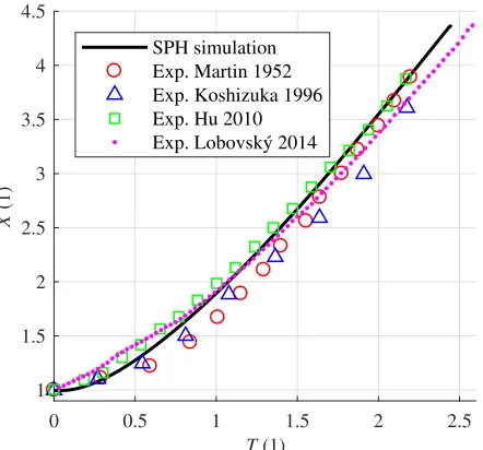
First, the surge front position obtained from the simu-lation was compared with experimental data from [1–3, 5] (Fig. 5). The computed position of surge front is in a rel-atively good agreement with all the experimental data.

(4)

0 0.5 1 1.5 2 2.5 T (1)

1 1.5 2 2.5 3 3.5 4 4.5

X

(1)

SPH simulation Exp. Martin 1952 Exp. Koshizuka 1996 Exp. Hu 2010 Exp. Lobovský 2014

Fig. 5. Non-dimensional surge front position as a function of non-dimensional time. Exp. Martin 1952 [1], Exp. Koshizuka 1996 [3], Exp. Hu 2010 [5], Exp. Lobovský 2014 [2].

0 2 4 6

T (1) 0

0.2 0.4 0.6 0.8 1

H

(1)

SPH simulation Exp. Lobovský 2014

Fig. 6. Non-dimensional liquid surface height as a function of non-dimensional time at position H1. Exp. Lobovský 2014 [2].

0 1 2 3 4 5 6

T (1) 0

0.05 0.1 0.15 0.2 0.25 0.3

H

(1)

0 1 2 3 4 5 6

T (1) 0

0.05 0.1 0.15 0.2 0.25

H

(1)

0 1 2 3 4

T (1) 0

0.05 0.1 0.15 0.2

H

(1)

in the simulation. The absence of the surrounding gaseous phase also plays its role [6].

The simulation is in a good agreement at positions H1 (Fig. 6), H2 (Fig. 7), and H3 (Fig. 8). However, a diff er-ence in a shape of the propagating wave is noticeable at positions H2 and H3 near T = 1.7 and T = 2 respec-tively. This difference further expands, and at position H4 (Fig. 9), the difference between the experiment and the simulation is quite significant. Again, this is possibly caused by the absence of viscosity and turbulence mod-elling.

3.2 Dynamics

Pressure was evaluated at four points P1 - P4 (see Fig. 1) placed on the right wall of the tank. Pressure is taken as a non-dimensional quantity

P= p

̺0|g|h0

, (22)

(5)

2 3 4 5 6 7 T (1)

0 0.5 1 1.5 2 2.5 3

P

(1)

Fig. 10. Non-dimensional pressure as a function of non-dimensional time at sensor P1. Exp. Lobovský 2014 [2].

2 3 4 5 6 7

T (1) 0

0.5 1 1.5 2

P

(1)

There is a sudden rise in pressure and the maximal value predicted by the simulation is about 10% higher than the experimental value. Then the pressure decreases and the simulation values remain above the experimental ones. At aboutT =6, there is a slight pressure rise in the experi-mental data. This rise occurs in the simulation as well, but later - at aboutT =6.5. It is so because this pressure rise is connected to the rolling wave impact, which occurs later in the simulation than in the experiment.

Pressure from sensor P2 is in Fig. 11. There is a peak in pressure value as in the previous case, but its amplitude is lower. The maximal value is very similar in the simu-lation and the experiment. However, the following drop of pressure values is lower in the simulation, and it stays about 20% above the values from the experiment. Just like in the previous case, the pressure rise appears later in the simulation than in the experiment, and it reaches slightly higher values.

2 3 4 5 6 7

T (1) 0

0.2 0.4 0.6 0.8 1 1.2 1.4 1.6

P

(1)

2 3 4 5 6 7

T (1) 0

0.2 0.4 0.6 0.8 1

P

(1)

The record from sensor P3 is shown in Fig. 12. The peak occurs again, but it is lower and wider than in the previous cases. The simulation predicts the maximal value about 25% lower than the maximal measured value, but it drops slower, and it stays up to 30% higher than the ex-perimental values. The pressure rise connected with the rolling wave impact occurs like in the previous cases.

(6)

4 Conclusion

In this work, a dam break problem was solved using a weakly compressible SPH method. The obtained results were compared with experimental data from the literature. The kinematics of the flow is in relatively good agreement with available experimental data, especially at the begin-ning of the problem solution. Later, an absence of vis-cosity and turbulence modelling becomes evident, partic-ularly during the formation of the rolling wave and dur-ing its impact. After the rolldur-ing wave impact, a neglection of the gaseous phase is not appropriate, as well as two-dimensional simplification because air remains trapped under the rolling wave in experiments, and it escapes in the form of bubbles.

The pressure was evaluated in four points on the right wall of the tank. In general, the deviation of simulation and experiment increased with the height above the bot-tom. Three lower placed sensors gave good quantitative agreement with the experiment with the maximal pressure value deviation up to 30%. The experimental and numer-ical data from the highest sensor differ considerably. A common feature for all sensors in both experiment and simulation is a pressure rise after the rolling wave impact; however, it occurs later in the simulation than in the exper-iments.

To suppress pressure field noise in the space domain, artificial diffusion and density reinitialization were imple-mented. Possible problems with the used artificial diff u-sion model have been reported for long-time hydrostatic simulation, but they did not occur in the solved problem [14]. For correct evaluation of the kinematics of the flow, a relatively coarse resolution is sufficient. However, domain of influence of a pressure sensor is resolution dependent and a finer resolution is necessary.

The output signal from the virtual pressure sensors was further filtered in the time domain. A filtering function which uses ’future’ values is employed since the time fil-tering is done after the computation. If the filtered val-ues were needed during the computation, different filter-ing function would have to be employed. The filterfilter-ing function and smoothing time period seem to be chosen correctly because high-frequency noise was mostly sup-pressed while sudden changes in pressure values, espe-cially steep rises after the impact, were captured properly.

Despite the simplicity of the model, the results are in relatively good agreement with the experiments. To ob-tain better results, viscosity and turbulence should be mod-elled. The two-dimensional simplification and neglection of the surrounding gaseous phase are not entirely correct as well, especially in the later phases of the simulation. Surface tension can also play its role when droplets and bubbles emerge.

This work was supported by the Grant Agency of the Czech Technical University in Prague, grant No. SGS18/124/OHK2/2T/12.

References

[1] J. C. Martin, W. J. Moyce, W. G. Penney, A. T. Price, C. K. Thornhill, Philos. Trans. A Math. Phys. Eng. Sci.244, 312-324 (1952)

[2] L. Lobovský, E. Botia-Vera, F. Castellana, J. Mas-Soler, A. Souto-Iglesias, J. Fluids Struct.48, 407-434 (2014)

[3] S. Koshizuka, Y. Oka, Nucl. Sci. Eng.123, 421-434 (1996)

[4] M. A. Cruchaga, D. J. Celentano, T. E. Tezduyar, Comput. Mech.39, 453-476 (2006)

[5] C. Hu, M. Sueyoshi, J. Marine Sci. Appl.9, 109-114 (2006)

[6] A. Colagrossi, M. Landrini, J. Comput. Phy.191, 448-475 (2003)

[7] A. Ferrari, M. Dumbser, E. Toro, A. Armanini, Com-put. Fluids38, 1203-1217 (2009)

[8] D. Laigle, M. Labbe, Int. J. Eros. Control Eng.10, 56-66 (2017)

[9] Z. Q. Zhou, J. O. De Kat, B. Buchner, Proc. 7th Int. Conf. Num. Ship Hydrod., 5.1. 1-15 (1999)

[10] J. J. Monaghan, J. Comput. Phys. 110, 399-406 (1994)

[11] D. Molteni, A. Colagrossi, Comput. Phys. Commun. 180, 861-872 (2009)

[12] S. Adami, X. Y. Hu, N. A. Adams, J. Comput. Phys. 231, 7057-7075 (2012)

[13] D. Shepard, ACM ’6823, 517-524 (1968)