Fully solvable mathematical scheme in finding out the right mass and width values of f0(500) and ρ0(770) mesons

Fully solvable mathematical scheme in finding out the right

mass and width values of

f0

(500)

and

ρ

(770)

mesons

StanislavDubnicka1∗and Anna ZuzanaDubnickova2

1_{Institute of Physics, Slovak Academy of Sciences, Bratislava, Slovakia} 2_{Department of Theoretical Physics, Comenius University, Bratislava, Slovakia}

Abstract. Starting from the phase representations with one subtraction of the pion scalar-isoscalar and vector-isovector charged pion electromagnetic form factor and exploiting the most accurate information on the S-wave isoscalar and the P-wave isovector ππ scattering phase shifts, respectively, to be ob-tained from the existing inaccurate experimental data by means of the Garcia-Kami´nski-Peláez-Yndurain Roy-like equations with an imposed crossing sym-metry condition, in the framework of the so-called "fully solvable mathematical scheme" the most reliable values of the f0(500) andρ0(770) meson mass and

width are found.

1 Introduction

If there is a function F(t) to be analytic in the whole complext-plane besides the cuts on the positive real axis from the lowest square root branch point t = 4 to +∞, fulfills the elastic unitarity condition ImF(t)= F(t)e−iδ_{sinδin elastic region withδto be some of the}

ππ scattering phase shifts, the asymptotic behavior F(t)|t|→∞ ∼ 1/t, the reality condition

F∗_(t)=F(t∗_{) and it is normalized att=0 to one, then one can write down using the Cauchy}

formula a dispersion relation with one subtraction at the point t = 0, which together with the unitarity condition through the Omnés-Muskelishvili integral equation leads to the phase representation ofF(t)

F(t)=Pn(t) exp

"_t

π

Z ∞

4

δ(t0₎

t0_(t0_−t)dt 0

#

(1) to be the starting point for our further investigations.

Under the "fully solvable mathematical scheme" [1] it is understood a procedure leading to a very simple form ofF(t) in the variable

q=[(t−4)/4]1/2 (2)

by means of an explicit calculation of the integral in the phase representation (1).

The functionF(t) on the positive real axis fort >4 is complex with the phaseδF to be

defined by the relation tanδF =

ImF(t)

ReF(t), (3)

which, however, due to the elastic unitarity condition, phenomenologically verified to be valid approximately up to 1 GeV, is identical with theππscattering phase shiftδ.

Since the transformation (2) is in fact a conformal mapping of the two-sheeted Riemann surface intvariable into oneq-plane, elastic cut, generated by the square root branch point

t=4, disappears.

Noticing the conformal mapping (2) in more detail, the first Riemann sheet intvariable, containing only branch points corresponding to opening various thresholds and zeros ofF(t), is mapped on the upper halfq-plane, whereby position of the branch pointt = 4 and the normalization pointt =0 are mapped intoq =0 andq = +i, respectively, and the real axis from−∞ up to t = 4, on which F(t) is a real function, is mapped on the whole positive imaginary axis of theq-plane.

The second Riemann sheet intvariable, containing branch points, again some zeros and also complex conjugate pairs of poles, which control the shape of F(t), is mapped on the lower halfq-plane.

If we restrict ourselves only to the elastic region and neglect contributions toF(t) of all inelastic branch points beyond 1 GeV, then there are only zeros in the upper and lower half

q-plane to be accounted as roots of a polynomial in numerator and conjugate pairs of poles according to the imaginary axis exclusively in the lower halfq-plane to be accounted as roots of a polynomial in denominator ofF(t).

As a result one can representF(t) in the form of the following rational function

F[t(q)]= PM

n=0anqn

PN r=0brqr

. (4)

Multiplying the numerator and denominator by the complex conjugate denominator, Eq. (4) is changed to the form

F[t(q)]=

PM+N s=0 csqs

(PN

r=0brqr)(PNr=0brqr)∗

. (5)

The reality conditionF∗(t)=F(t∗) results in the reality of (5) on the positive imaginary axis of theq-plane. Then it is straightforward to see that the expression

F[t(q)]=(c0+c2q 2_+c

4q4+...)+i(c1q+c3q3+c5q5+...) (PN

r=0brqr)(PNr=0brqr)∗

(6) actually fulfils the latter claim and through the definition of the phase ofF(t) leads to the following parametrization of theππscattering phase shiftδ

δ=arctanA1q+A3q 3_+A

5q5+A7q7+... 1+A2q2+A4q4+A6q6+...

, (7)

with all coefficients to be real. This parametrization is derived directly from the basic princi-ples like analyticity, unitarity and reality condition.

2 Pion scalar-isoscalar form factor and

f

(500)

meson parameters

The pion scalar-isoscalar form factor (FF)Γπ(t) is defined by the matrix element of the scalar quark density

witht=(p2−p1)2and ˆm=1₂(mu+md), and fulfils all properties of the functionF(t) defined

in Sect.1. Even the normalization of physically nonmeasurable pion scalar FFΓπ(t) is equal to one as it is seen from the calculated pion sigma term value with error

Γπ(0)=(0.99±0.02)m2π (9)

in the framework of theχPT [2], if the pion massmπis taken to be one.

Then the phase representation of the pion scalar-isoscalar FF is Γπ(t)=Pn(t) exp

      t π

Z ∞

4

δ0 0(t

0₎

t0_(t0_−t)dt 0

    

, (10)

whereδ0

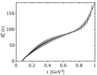
0(t) is now the S-wave isoscalarππscattering phase shift to be exactly equal to the parametrization (7) with the parameterA1to be identified with the S-wave isoscalarππ scat-tering lengtha0₀. The number of nonzero parameters in (7) and their numerical values are found in a fitting procedure of the most precise data onδ0₀(t) with theoretical errors in Fig.1

to be generated by Garcia-Kami´nski-Peláez-Yndurain (GKPY) equations [3] for the S-wave isoscalarππscattering amplitude.

Figure 1. The data onδ0

0(t) with theoretical errors to be generated by GKPY equations for the

S-wave isoscalarππscattering amplitude. Solid line represents our optimal fit of data with 5 nonzero coefficientsAiin (7)

The data in Fig.1have been analyzed by the relation (7) up to the moment, when the min-imum ofχ2_{/ndf was achieved. The latter has been found with the first 5 nonzero coefficients}

Aiof the values

A1 = 0.2219±0.0029

A2 = −0.0764±0.0423

A3 = 0.1390±0.0251

A4 = −0.0062±0.0053

A5 = −0.0135±0.0020

and the final form of the S-wave isoscalarππscattering phase shiftδ0

0(t) takes the form

δ0

0(t)=arctan

A1q+A3q3+A5q5 1+A2q2+A4q4

Substitution of (11) into (10), however, leads to the expression which does not allow one to calculate the corresponding integral explicitly.

Therefore we have used the equivalent form

δ0 0(t)=

1 2iln

"

(1+A2q2+A4q4)+i(A1q+A3q3+A5q5) (1+A2q2+A4q4)−i(A1q+A3q3+A5q5) #

(12) to (11) to be valid in the theory of functions of complex variable.

The latter leads to

Γπ(t)=Pn(t) exp

         

(q2+1) 2πi

Z ∞

−∞

q0_ln(1+A2q02+A4q04)+i(A1q0+A3q03+A5q05)

(1+A2q02+A4q04)−i(A1q0+A3q03+A5q05)

(q02+_1)(q02_−q2₎ dq

0           , (13)

and the integral in (13)

I= Z ∞

−∞

q0ln(q0−q1)(q0−q2)(q0−q3)(q0−q4)(q0−q5)

(q0_−q∗

1)(q

0_−q∗

2)(q

0_−q∗

3)(q

0_−q∗

4)(q

0_−q∗

5)

(q0+_i)(q0_−i)(q0+_ib)(q0_−ib) dq

0_{, (14)}

with

q2<0 i.e. q=i r

4−t

4 ≡ib and

q1 = 0.00 −i2.0430±0.2029, q∗₁ = −q1,

q2 = 1.41470±0.0579 +i1.0749±0.0162, q∗₂ = −q3,

q3 = −1.4147±0.0579 +i1.0749±0.0162, q∗₃ = −q2,

q4 = 3.3827±0.0115 +i0.1744±0.0340, q∗₄ = −q5,

q5 = −3.3827±0.0115 +i0.1744±0.0340, q∗₅ = −q4

(15)

now can be calculated in the framework of the theory of residue explicitly.

In order to carry out it practically, it is convenient to decompose the integral (14) into a sum of two integrals

I=I1+I2= Z +∞

−∞

q0ln(q0−q2)(q0−q3)(q0−q4)(q0−q5)

(q0_−q∗

1)

(q0_+i)(q0_−i)(q0_+ib)(q0_−ib)dq

0_{+ (16)}

         − Z −∞ +∞

q0_ln (q0_−q

1)

(q0_−q∗

2)(q

0_−q∗

3)(q

0_−q∗

4)(q

0_−q∗

5)

(q0+_i)(q0_−i)(q0+_ib)(q0_−ib)dq 0         

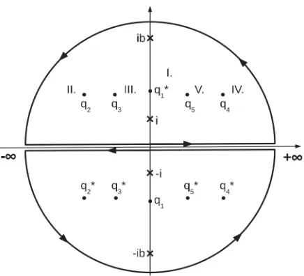
according to singularities to be placed in the upper or lower halfq-plane, as it is sketched in Fig.2.

Then the explicit form of

I= 2πi

(q2+₁₎ln

(q−q∗₁)

(q−q∗₂)(q−q∗₃)(q−q∗₄)(q−q∗₅)

(i−q∗₂)(i−q∗₃)(i−q∗₄)(i−q∗₅) (i−q∗₁)

! (17) is obtained in the straightforward way, if in the case of the first integral

I

φ1(q0)dq0=2πi

2 X

n=1

Figure 2.Poles (×) and branch points (•) of the integrandsφ1(q0) andφ2(q0) with contours of

integra-tions in the upper and the lower halfq-planes, respectively

the contour of integration is closed in the lower halfq-plane and in the second integral I

φ2(q0)dq0=2πi 2 X

n=1

Resn (19)

the contour of integration is closed in the upper halfq-plane (see Fig.2).

In a such way one avoids complicated calculations of the cut-contributions to be auto-matically generated by branch points under logarithms, if the contours are drawn as it is demonstrated in Fig.2.

The substitution of (17) into (13) leads to the explicit form of the pion scalar-isoscalar FF Γπ(t)=Pn(t)

(q−q∗

1) (q−q∗

2)(q−q

∗

3)(q−q

∗

4)(q−q

∗

5)

(i−q∗₂)(i−q∗₃)(i−q∗₄)(i−q∗₅) (i−q∗

1)

, (20)

wherePn(t) is any polynomial normalized att = 0 to one, however, it has not violate the

asymptotic behavior of the pion scalar-isoscalar FF. The poleq = q∗

3 on the second Riemann sheet int-variable corresponds to the f0(500) meson resonance, now with the mass and the width,mσ=(459±29) MeV andΓσ=(517±

77) MeV [7], respectively, which are compatible with the parameters obtained in [4,5]. The Rev. Part. Physics (2016) [6] gives parameters of f0(500) to be mσ = (400−

550) MeV andΓσ=(400−700) MeV.

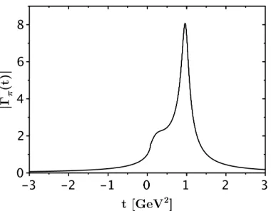
A behavior of theΓπ(t) (20) at−3 GeV2<t<3 GeV2is presented in Fig.3.

3 Vector pion electromagnetic form factor and

ρ

(770)

meson

parameters

The vector isovector charged pion electromagnetic (EM) form factorFπE M,I=1(t) is defined by

the matrix element of the pion EM currentJE M

µ as follows

Figure 3.Behavior of the pion scalar form factor (20) with one zero and four poles at−3 GeV2 <t< 3 GeV2_{. Results correspond to a fit to the output phase shifts from [3] by 5 free parameters. Physically}

may be interpreted region only below 990 MeV (t≈0.98 GeV2₎

witheto be the electric charge andt = (p2−p1)2 the momentum transfer squared. The

FπE M,I=1(t) also fulfils all properties of the function F(t) defined in Sect. 1, including the

normalizationFπE M,I=1(0)=1, if the electric charge is put to be one. ThenFπE M,I=1(t) can be represented by the phase representation

FπE M,I=1(t)=Pn(t) exp

      t π

Z ∞

4

δ1 1(t

0₎

t0_(t0_−t)dt 0

    

, (22)

whereδ1₁(t) is now the P-wave isovectorππscattering phase shift and Pn(t) is polynomial

normalized att=0 to one, however, it has not violate the asymptotic behavior of the charged pion EM FF.

In this case the model independent parametrization (7), taking into account a threshold behavior of theδ1

1(t)|q|→0∼a11q

3_{, has to be adapted to the form}

δ1

1(t)=arctan

A3q3+A5q5+A7q7+... 1+A2q2+A4q4+A6q6+...

, (23)

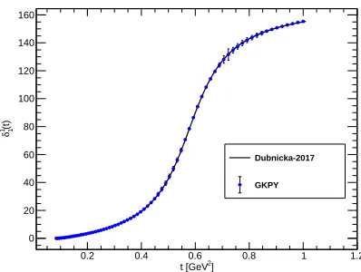
where the parameterA3is identified with the P-wave isovectorππscattering lengtha1₁. The number of nonzero parameters in (23) and their numerical values are again found in a fitting procedure of the most precise data onδ1₁(t) with theoretical errors in Fig.4to be generated by Garcia-Kami´nski-Peláez-Yndurain equations [3] for the P-wave isovectorππ scattering amplitude.

The minimum ofχ2_{/ndf was achieved by the first 4 nonzero values of coefficients in (23)}

A2 = 0.1070±0.0329

A3≡a11 = 0.0321±0.0008

A4 = −0.03825±0.0030 (24)

0.2 0.4 0.6 0.8 1 1.2 ]

2 t [GeV 0

20 40 60 80 100 120 140 160

(t)

1_δ1

Dubnicka-2017

GKPY

Figure 4.Optimal description of the GKPYδ1

1(t) data. Solid line represents our optimal fit of data with

4 nonzero coefficientsAiin (23)

and the roots of the corresponding polynomials in the numerator and denominator of the equivalent to (23) logarithmic relation

δ1 1(t)=

1 2iln

"₍₁+_A

2q2+A4q4)+i(A3q3+A5q5) (1+A2q2+A4q4)−i(A3q3+A5q5) #

(25) are

q1 = −2.5480±0.0020 +i0.2752±0.0016, q∗₁ = −q2,

q2 = 2.5480±0.0020 +i0.2752±0.0016, q∗₂ = −q1,

q3 = 0.0 −i1.8432±0.0658, q∗₃ = −q3,

q4 = 0.0 +i2.146±0.1054, q∗₄ = −q4,

q5 = 0.0 −i139.793±0.152542, q∗₅ = −q5.

(26)

A substitution of (25) with (26) into (22) leads to

F_πE M,I=1(t)=Pn(t) exp

" (q2₊₁₎

2πi Z ∞

−∞

(q0_−q1)(q0_−q2)(q0_−q3)(q0_−q4)(q0_−q5)

(q0_−q∗

1)(q0−q

∗

2)(q0−q

∗

3)(q0−q

∗

4)(q0−q

∗

5)

dq0 #

(27) and the integral in (27) is calculated in the same way as it was done in the case of the scalar-isoscalar pion FF.

The poleq =q∗

1 on the second Riemann sheet int-variable corresponds to theρ 0₍₇₇₀₎ meson resonance, with the mass and the width,mρ =(763.56±0.51) MeV andΓρ=(143.09±

0.82) MeV [7], respectively.

The Rev. Part. Physics (2016) [6] gives parameters of ρ0_{(770) to be m}

ρ = (775.26±

0.25) MeV andΓρ=(149.1±0.8) MeV.

4 Conclusions

most accurate up to now information on the S-wave isoscalar and the P-wave isovectorππ scattering phase shifts, respectively, to be obtained from the existing inaccurate experimental data by means of the Garcia-Kami´nski-Peláez-Yndurain Roy-like equations with an imposed crossing symmetry condition, in the framework of the so-called "fully solvable mathemati-cal scheme" the most reliable values of the f0(500) andρ0(770) meson mass and width are determined.

The work was supported by VEGA grant No.2/0153/17.

References

[1] S. Dubnicka, A.Z. Dubnickova and A. Liptaj, Phys. Rev. D90, 114003 (2014) [2] J. Gasser and U-G. Meissner, Nucl. Phys. B357, 90 (1991)

[3] R. Garcia-Martin, R. Kami´nski, J.R. Pela’ez, J. Ruiz de Elvira and F.J. Yndurain, Phys. Rev. D83, 074004 (2011)

[4] I. Caprini, G. Colangelo and H. Leutwyler, Phys. Rev. Lett.96, 132001 (2006)

[5] R. Garcia-Martin, R. Kami´nski, J. R.Pela’ez and J. Ruiz de Elvira, Phys. Rev. Lett.107, 072001 (2011)

[6] C. Patrignani et al. [Particle Data Group],Review of Particle Physics, Chin. Phys. C40, 100001 (2016)