692 | P a g e
INTEGRATION OF INVENTORY CONTROL AND
SCHEDULING USING BINARY PARTICLE SWARM
OPTIMIZATION ALGORITHM
Manash Dey
Assistant Professor, Mechanical Engineering Department, JIMS EMTC Greater Noida (India)
ABSTRACT
Production planning and scheduling are usually performed in a hierarchical manner, thus generating unfeasibility
conflicts when comes to implementation. Moreover, solving these problems simultaneously in complex
manufacturing systems is very challenging in production management. Production planning is first performed at the
tactical decision level and, the different jobs are then supposed to be scheduled at the operational decision level.
Therefore, the information about capacity planned at the tactical level is in aggregate manner, thus not
guaranteeing that scheduling constraints are respected. Thereby, the production plans may be unfeasible.
An integrated approach for guaranteeing consistency to some extent between decisions taken at tactical and operational levels of production management was presented, thus avoiding the shortcomings of traditional
approaches in which decisions are taken sequentially. Integrated problem are solved by using the exact capacity
constraint from a standard scheduling problem to the lot sizing problem.
However this combinatorial optimization problem can be solved by using soft computing techniques in reasonable
time. In the present work we have applied Binary Particle Swarm optimization (BPSO) technique to the Single item
single level, multi-level and Multi item Lot sizing problems with and without applying the Scheduling constraint. We
have tested the BPSO technique to the different types and sizes of problems by applying scheduling constraint. The
obtained results are compared with Lot sizing problems without constraint and it is concluded that in all instances the results are improved compared to simple lot sizing problems.
Keywords: MRP, Binary Particle Swarm optimization (BPSO)
I. INTRODUCTION
693 | P a g e
excess inventories of other products. This raises the issue of finding the right balance between cutting costs and maintaining customer responsiveness. Previously, production specialists used multiple and sometimes contradictory or confusing databases, data gathered from machine operators, and past experience to gauge what was needed to meet production goals. Problems always take place on shop floor when generating MRP and production schedule are separately taken into account since both MRP and schedule aim for different objectives which are not synchronized. MRP is computer software based production planning and inventory control system used to ensure that all materials required are ready for production and requested products are available for delivery to customers with the lowest possible level of inventory. Using conventional MRP and classic shop floor scheduling separately cannot solve the problem. Integration of inventory control and scheduling is one of the solutions.II. MATHEMATICAL FORMULA
1. Mathematical formulation to the Single level Lot sizing Problem (SISL)
The incapacitated single item no shortages allowed and single level lot sizing model is the simplest model in the inventory lot sizing problems. Lot sizing formulation for this kind of lot sizing problem takes the following form
Where
694 | P a g e
2. Mathematical formulation to the Multi level Lot sizing Problem (MLLS)
1 1 , 1 ( )
min
(
)
(1)
(2)
(3)
0,
{0,1}
(4)
0,
0
(5)
P T
i it i it i t
it i t it it it ij jt
j i
it it it it it
s y
h I
I
I
x
d
d
c x
x
My
y
I
x
Necessary notations:Γ (i): set of immediate successors of items i; Γ -1(i): set of immediate predecessors of items i; c
ij : quantity of item i
required to produce one unit of items j; Di,t : external requirement for items i in period t; hi: holding cost for items i
(Following small instance standard); Ii,0 : initial inventory of product i; Si : setup cost for items i (Following small
instance standard); T: total number of periods. Decision and auxiliary variables:
di,t : total requirement for item i in period t; Ii,t : Inventory level of item i at the end of period t; Xi,t: delivered
quantity of items i at the beginning of the period t; Yi,t: binary variable which indicates if an item i is produced in
period t, (yi,t = 1 ) or not (yi,t = 0 ).
3. Integrated formulation of planning and scheduling
The problem is formulated as
1 1
1 1
min
(
.
.
.
)
(
)
(
)
0,
1,... ;
1,...,
(1)
0,
,
(2)
0,
,
(3)
0,
,
(4)
.
0, (
,
)
(5)
T n
pr it it it it it it t i
it it it it it it it
it it
u
ijkt ij k t ij k t it ij k t ijkt
c I
c I
c
X
I
I
I
I
X
D
i
n t
T
X
i t
I
i t
I
i t
t
t
p
X
o
o
A
t
1 1 10,
(6)
.
0, (
,
)
( )
(7)
.
,
(8)
.
,
(9)
ijkt ijkt u
ijkt i j kt i j kt i t i j kt ijkt t
u
ijkt ijkt it l ijkt l
t u
ijkt ijkt it l ijkt l
o
N
t
t
p
X
o
o
S y
t
p
X
c
o
L
t
p
X
c
o
L
695 | P a g e
The objective function in the above problem is the minimization of sum of the Inventory surplus, backlog, and production cost of the products to be planned. (1) is the standard inventory balance equation. Constraints 2, 3, 4 presents that production items, inventory surplus, backlog quantities are always positive. Constraint 5 gives the conjunctive constraint relationship among the operation on the machines. (6) Gives that starting times of operation Oijt are always positive. Constraints 7 give disjunctive constraints relations among the operations. Constraints 8 & 9 state that the last operations of the Jit must be completed in period t and not before. Constraint 7 replaced with necessary conditions which does not involve Disjunctive constraints.III. IMPLEMENTATION OF BPSO TO INTEGRATED PROBLEM
1. Binary Particle Swarm Optimization Algorithm (BPSO)
Pseudo code of the general PSO is given as
2. 3. 4. 5. 6. 7. 8. 9. 10. 11.
The basic elements of PSO algorithm is summarized as follows:
Particle: is a candidate solution i in swarm at iteration k. The ith particle of the swarm is represented by a d-dimensional vector and can be defined as Xik =[Xki1, Xki2, Xki3…. Xkid], where x’s are the optimized parameters and
Xkid is the position of the ith particle with respect to dth dimension. In other words, it is the value dth optimized
parameter in the ith candidate solution.
Population: popk is the set of n particles in the swarm at iteration k, i.e., popk=[ X1k, X2k, X3k……… Xnk].
1 1
(
.
)
ijkl kl
t t
u
ijkl il l
l o O l
P
X
C
Begin
Step 1: Initialization
Initialize swarm, including swarm size, each particle’s position
and velocity;
Evaluate the each particle fitness;
Initialize gbestposition with particle with the lowest fitness in the
swarm;
Initialize pbest position with a copy of particle itself;
Give initial value: W
max,W
min,C
1,C
2and generation=0;
Step 2: Computation
While (the maximum of generation is not met)
Do {
Generation++;
Generate next swarm by equation (1a) and (1b);
Evaluate Swarm
{
Find new gbest and pbest;
Update gbestof the swarm and pbest of each particle;
}
}
696 | P a g e
Particle velocity: Vik is the velocity of particle i at iteration k. It can be described as Vik = [Vki1,Vki2,Vki3….Vkid],where Vidk is the velocity with respect to dth dimension.
Particle best: PBi k
is the best value of the particle i obtained until iteration k. The best position associated with the best fitness value of the particle i obtained so far is called particle best and defined as PBi
k
= [pbki1,
pbki2,pb k
i3….pb k
id], with the fitness function f(PBi k
).
Global best: GBik is the best position among all particles in the swarm, which is achieved so far and can be
expressed as GBik = [gbki1, gbki2,gbki3….gbkid], with the fitness function f(GBik).
Termination criterion: it is a condition that the search process will be terminated. In this study, search is terminated when the number of iteration reaches a predetermined value, called maximum number of iteration.
The complete computational flow of the binary PSO algorithm is given below:
Step 1: Initialization
a) Set k=0, n=twice the number of dimensions
b) Generate n particles randomly as, {Xi0,i=0,1,2,……n},where Xi0 =[X0i1, X0i2, X0i3…. X0id].
c) Generate the initial velocities of all particles randomly, {Vi0,i=0,1,2,……n}, where Vi0 =[v0i1, v0i2, v0i3….
v0id]. v0id is randomly generated with vid=Vmin+( Vmax - Vmin)*rand().
d) Evaluate each particle in the swarm using the objective function, f(Xi0).
e) For each particle i in the swarm, set PBi0= Xi0,where PBi0 = [pb0i1= X0i1, pb0i2= X0i2, pb0i3= X0i3….. pb0id=
X0id along with its best fitness value, fipbest(PBi0,i=1,2,3….n).
f) Set the global best to, , figbest(GB0)=min{ fipbest(PBi0,i=1,2,3….n)} with GB0=[gb1, gb2,… gbd]
Step 2: Update iteration counter
k=k+1
Step 3: Update velocity by using the piece-wise linear function
h
C1 and C2 are social and cognitive parameters and r1 and r2 uniform random numbers between (0, 1).
Step 4: Update dimension (position) by using the sigmoid function
Xidk={1, if U(0,1)<sigmoid (vkid)
0, otherwise
697 | P a g e
Each particle is evaluated again with respect to its updated position to see if particle best will change. That is,
If fik(Xik,i=0,1,2,……n) < fipbest(PBik-1,i=0,1,2,……n)
then
fipbest(PBik,i=0,1,2,……n) = fik(Xik,i=0,1,2,……n)
else
fipbest(PBik,i=0,1,2,……n) = fipbest(PBik-1,i=0,1,2,……n)
Step 6: Update global best
fgbest(GBk) = min { fipbest(PBik,i=1,2,……n)}
if fgbest(GBk)< fgbest(GBk-1), then fgbest(GBk) = fgbest(GBk)
else fgbest(GBk) = fgbest(GBk-1) Step 7: Stopping Criterion
If the number of iteration exceeds the maximum number iteration, then stop, otherwise go to step 2.
IV. RESULT
1.
Single item Multi level Problem
1
2
3
7
6
5
4
698 | P a g e
Table 1.1 Demand of products and cost involved in (7×6) problem
Period 1 2 3 4 5 6
Problem76 25 20 15 10 20 35
Item no 1 2 3 4 5 6 7
S.C 400 500 1000 300 200 400 100
H.C 12 0.6 1 0.04 0.03 0.04 0.04
Table 1.2 Demand of products for three different problems
period 1 2 3 4 5 6 7 8 9 10 11 12
Demand 25×12
15 5 15 110 65 165 125 25 90 15 140 115
Demand 40×12
10 100 10 130 115 150 70 10 65 70 165 25
Demand 50×12
15 5 15 120 65 155 125 25 95 15 135 115
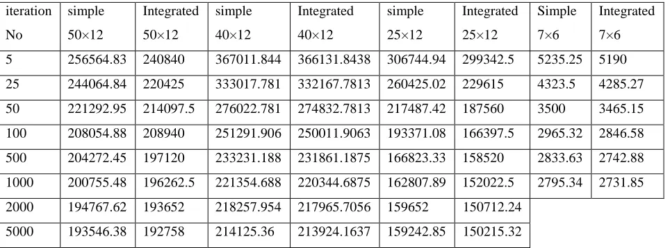
Comparison of results with and without scheduling constraint tested at different iterations
Table 1.3 SIML problem solution with four different sizes at different iterations
iteration No
simple 50×12
Integrated 50×12
simple 40×12
Integrated 40×12
simple 25×12
Integrated 25×12
Simple 7×6
Integrated 7×6 5 256564.83 240840 367011.844 366131.8438 306744.94 299342.5 5235.25 5190 25 244064.84 220425 333017.781 332167.7813 260425.02 229615 4323.5 4285.27 50 221292.95 214097.5 276022.781 274832.7813 217487.42 187560 3500 3465.15 100 208054.88 208940 251291.906 250011.9063 193371.08 166397.5 2965.32 2846.58 500 204272.45 197120 233231.188 231861.1875 166823.33 158520 2833.63 2742.88 1000 200755.48 196262.5 221354.688 220344.6875 162807.89 152022.5 2795.34 2731.85 2000 194767.62 193652 218257.954 217965.7056 159652 150712.24
699 | P a g e
Figure 1.1 Convergence of Four SIML problems solutions at different iterations
2.
Multi item level Problem
Table 1.4 MIML problem solution with three different sizes at different iterations
iteration no
Simple 39×12
Integrated 39×12
Simple 15×12
Integrated 15×12
Simple 25×12
Integrated 25×12 5 422388.1563 412894.2812 267876.5625 252053.1563 350988.8125 336092.2813 25 376876.25 365135.0937 204949.6563 194649.6563 293958.2188 283658.2188 50 340013.4688 328273.875 163244.7031 156844.7031 236183.5313 222883.5313 100 280418.8438 267891.5937 124069.1641 123669.1641 194280.3594 189580.3594 200 255216.375 244539.421 121145.0547 120225.8984 181030.5625 175430.5625 500 244271.6406 231291.8906 113352.3047 112148.213 170112.3906 166256.7813 1000 230098.312 223192.4062 103500.2031 101742.2361 156994.7188 154257.6875 2000 222510 213361.4687 100472.1862 94232.80469 155365.7031 150367.7969
700 | P a g e
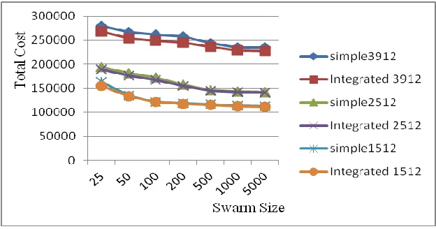
Figure 5.9 Comparison of three MIML problems solutions at different iterations
Figure 5.6 Convergence of three SIML problems solutions at different Swarm sizes
701 | P a g e
V. CONCLUSIONS
To the best of knowledge no work related to the integration problem by using BPSO technique has been published so far in the contemporary literature. BPSO technique have been successfully applied to integrated model and tested for different lot sizing problems such as single item single level, single item multi-level and multi item problems with three different product structures. In all the problem instances we found the improvement in inventory cost by introducing the scheduling constraint in the lot sizing problems. We found that problem solutions are converging at higher number of iterations and Swarm sizes.
Computational experience of BPSO algorithm to the combinatorial optimization problems in manufacturing decision making problems is good and its implementation to manufacturing problems is easy as it is having few number of control parameters in algorithms compared to other evolutionary algorithms.
REFERENCES
[1]. Staggemeier, A.T., et Clark, A.R.: A survey of lot-sizing and scheduling models, 23rd Annual Symposium of the Brazilian Operational Research Society, (2001) 603-617.
[2]. M. Fatih Taşgetiren & Yun-Chia Liang, a binary particle swarm optimization algorithm for the lot sizing problem, Journal of Economic and Social Research 5 (2), 1-20.
[3]. Wagner H. M and Whitin T. M, “Dynamic Version of the Economic Lot Size Model”, Management Science, Vol. 5, 1958.
[4]. Kennedy J. and Eberhart R. C., “A Discrete Binary Version of the Particle Swarm Optimization”, Proc. Of the conference on Systems, Man, and Cybernetics SMC97, pp. 4104-4109, 1997.
[5]. Klorklear Wajanawichakon1† , Rapeepan Pitakaso2, Solving large unconstrainted multi level lot-sizing problem by a binary particle swarm optimization, International Journal of Management Science and Engineering Management, 6(2): 134-141, 2011.
[6]. Afentakis. P. and Gavish. B, (1986). Optimal lot-sizing algorithms for complex product structures. Operation Research, 34(2):237–249.
[7]. N.P. Dellaert a, J. Jeunet, Randomized multi-level lot-sizing heuristics for general product structures, European Journal of Operational Research 148 (2003) 211–228.
[8]. Kennedy, J., Eberhart, R., and Shi, Y. (2006). Swarm intelligence. Handbook of Nature-Inspired and Innovative Computing, 187–219.
[9]. Fleischmann B & Meyr H, The General Lot sizing and Scheduling Problem, OR Spektrum 19,Vol. 1, pp. 11-21, 1997.
702 | P a g e
[11]. Meyr H, Simultaneous Lot sizing and Scheduling by Combining Local Search with Dual Reoptimization,European Journal of Operational Research 120, pp 311-326, 2000.
[12]. Drexl A & Kimms A, Lot sizing and scheduling - Survey and extensions, European Journal of Operational Research 99, pp 221-235, 1997.
[13]. Kimms A, A genetic algorithm for multi-level, multi-machine lot sizing and scheduling, Computers & Operations Research 26, pp. 829-848, 1999.
[14]. Héla OUERFELLI, Abdelaziz DAMMAK, Emna KALLEL CHTOUROU / Benders-based approach for an integrated Lot-Sizing and Scheduling problem. © International Journal of Combinatorial Optimization Problems and Informatics, Vol. 3, No. 3, Sep-Dec 2012.