ABSTRACT
GARUD, HRISHIKESH DEEPAK. Transforming Human Pose Forecasting. (Under the direction of Dr. Tianfu Wu).
Computational understanding of human pose has been under a high degree of scrutiny
recently, resulting in subsequent innovation. Particularly, the efforts to forecast human
pose in a temporal setting using Recurrent Neural Networks have gained significant
trac-tion chiefly because of improvements in these networks (read: Long Short Term Memory
units and/or Gated Recurrent Units) and an improved understanding of the learned
latent representation of data (read: Encoder-Decoder framework).
In this work, we analyze the important questions surrounding this interesting
com-puter vision problem, formulate the mathematical basis, study a novel neural network
architectural paradigm for language modeling - The Transformer, and explore its via-bility for human pose forecasting as a sequence-to-sequence learning scheme. We train
the system end-to-end to predict the future pose by combining the latent representation
for images with normalized-encoded pose information, jointly regressing over this latent
© Copyright 2019 by Hrishikesh Deepak Garud
Transforming Human Pose Forecasting
by
Hrishikesh Deepak Garud
A thesis submitted to the Graduate Faculty of North Carolina State University
in partial fulfillment of the requirements for the Degree of
Master of Science
Electrical Engineering
Raleigh, North Carolina
2019
APPROVED BY:
Dr. Edgar Lobaton Dr. Xu Xu
Dr. Tianfu Wu
DEDICATION
ACKNOWLEDGEMENTS
This thesis would not have been possible without the help and support of my advisor,
Dr. Tianfu Wu. From the very beginning of my Masters, he played a critical role in
shaping my research acumen and critical thinking. His unrelenting push to improve the
bar by setting high expectations and his dedication to his students make him a wonderful
advisor.
I appreciate the work put in by Dr. Edgar Lobaton and Dr. Xu Xu in patiently
reviewing my thesis. Dr. Lobaton was also instrumental in imbibing an interest and curiosity for this field through his enthusiastic lectures and detailed notes on the subject.
I also acknowledging the unwavering drive and encouragement from from my family
TABLE OF CONTENTS
List of Tables . . . v
List of Figures . . . vi
Chapter 1 Introduction . . . 1
1.1 Motivation . . . 1
1.2 Challenges in Human Gait . . . 2
1.3 Thesis contributions and structure . . . 3
Chapter 2 Background . . . 6
2.1 Related Work . . . 6
2.2 The Transformer . . . 8
2.2.1 Encoder and Decoder . . . 9
2.2.2 Attention Mechanism . . . 10
2.2.3 Positional Embedding . . . 14
2.2.4 Feed-Forward Network . . . 15
2.2.5 Layer vs. Batch Normalization . . . 15
2.3 Variational Encoder . . . 16
Chapter 3 Methodology . . . 18
3.1 Problem Formulation . . . 18
3.2 Data . . . 19
3.2.1 Dilated Sliding Window . . . 20
3.2.2 Strided Sliding Window . . . 20
3.3 Experiments . . . 21
3.3.1 Naive Pose Forecasting . . . 21
3.3.2 Pose Forecasting using Global Context . . . 21
3.4 Preprocessing . . . 21
3.5 Optimizer and Learning Rate Schedule . . . 22
3.6 Loss function and Evaluation Metric . . . 22
3.7 Hardware and Training Schedule . . . 23
Chapter 4 Results . . . 24
4.1 Ablations . . . 24
4.1.1 Change in network structure . . . 24
4.1.2 With global image context . . . 27
Chapter 5 Conclusions . . . 31
LIST OF TABLES
LIST OF FIGURES
Figure 1.1 Correlation matrix for x-coordinates of joints during a Baseball Pitch 3
Figure 1.2 Correlation matrix for x-coordinates of joints during a Pull-up . . 4
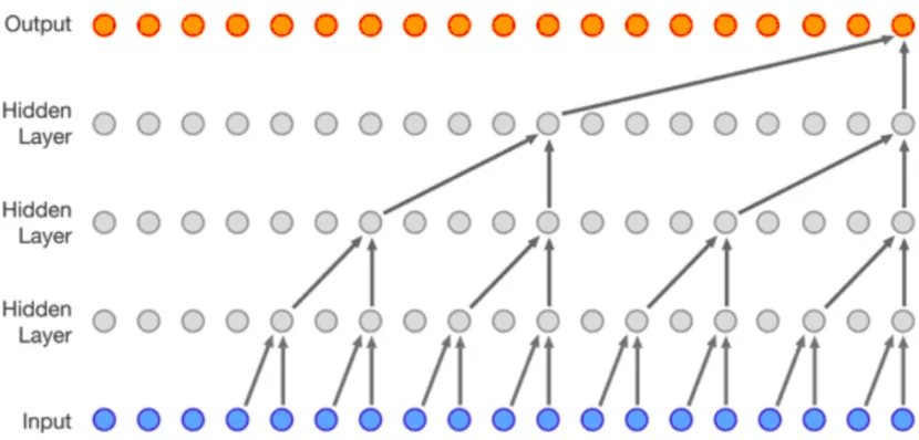
Figure 1.3 Correlation matrix for x-coordinate of joints for all training data 5 Figure 2.1 The WaveNet structure - a fully convolutional network with varying dilation factors allowing it to cover a number of timesteps . . . 8
Figure 2.2 The ByteNet structure - the decoder (blue part) is dynamically unfolded so that it is conditioned on the representations of the input sequence produced upto the present step. . . 9
Figure 2.3 The Transformer structure . . . 10
Figure 2.4 Self-Attention mechanism structure . . . 13
Figure 2.5 Three ways of Attention . . . 14
Figure 2.6 Positional Embeddings using sine and cosine waves. . . 15
Figure 3.1 Penn Action Dataset sample . . . 19
Figure 4.1 Transformer(BIG) vs LSTM - PCK and MSE on the test set . . . 25
Figure 4.2 Transformer(BASE) vs LSTM - test PCK and MSE using image context . . . 28
Figure 4.3 Baseball Pitch short-term forecasting . . . 28
Figure 4.4 Baseball Pitch long-term forecasting . . . 29
Figure 4.5 Golf swing short-term forecasting . . . 29
Chapter 1
Introduction
1.1
Motivation
Our decades old technological push towards achieving Singularity has led us to develop
artificial intelligence systems which can mimic human decision making up to a certain
degree. From simple classification tasks (10) to beating humans at Jeopardy (15) and Go (43)(44), we have come a long way in the progress to achieving Artificial
Super-intelligence in the form of General AI. One such active area of research is teaching
machines to understand the high degree-of-freedom configuration of human skeletal pose.
There have been recent advances in pushing the state-of-the-art for pose estimation
and detection in real time (39)(14)(28)(51)(37)(4)(52)(45). Usually, these systems are
trained to output the 2-D (or in some cases 3D) coordinates of various key-points of
the skeleton when the input is a RGB image containing n ≥ 1 human subjects with
varying degrees of difficulty in terms of shadows, occlusion and scale. Apart from an
interesting computer vision problem to solve, the application scope for real-time human pose detection/estimation is ideally suited for research in sport sciences to study and/or
to improve athletic performance or applied to gaming and animation.
An interesting extension to this domain will be to train a system to actually
pre-dict/forecast human pose in a temporal setting. This research is especially important
and necessary citing the surge in progress for robot autonomy and autonomous
vehi-cles research involving a high degree of dynamic human-machine cohabitation. These
autonomous agents need to be able to predict and forecast human dynamics in order to
improve their decision making and accelerate growth towards a fully autonomous
wasteful latencies in cognitive processing.
1.2
Challenges in Human Gait
What makes this area so difficult, apart from the multi-modality of the domain space, is
the fact that there is a lot of variation involved in various human body poses for various
activities. No human, performing the same activity, moves in the exact same manner
again. Add to it the dynamic uncertainty of a temporal prediction problem, resulting in
the domain space becoming infinitely more complicated.
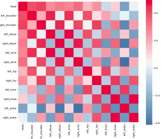
Another tricky aspect in trying to forecast human pose is the physical and dynamic constraints on human gait. Consequently, a subset of all body joints move in tandem
during a particular activity. This results in a high degree of correlation between these
joints which is reflected in the correlation matrix of the x and y coordinates of these
joints in the image plane.
The Pearson Correlation Coefficient(41) is an effective and a simple way to gauge the
relationship between feature vectors.
Figures 1.1 to 1.3 are best viewed in color.
Figure 1.1 shows the correlation between human joints when the skeleton goes through
a baseball pitch. As the activity entails positions and functions performed independently by the joints, we see a wider spread of influence for a particular keypoint.
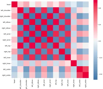
Meanwhile, in figure 1.2 we observe a more localized dependence between select few
human joints. The activity observed for this instance is a human doing Pull-up exercises.
As majority of body parts move together while doing a pull-up, a high correlation is
observed for those few joints.
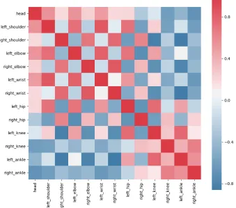
When we look at the entire training data, figure 1.3 clearly shows the relationship is
more generalized. However, on closer inspection, we still find points 1 through 7 are more
closely related than points 8 through 12.
In machine learning echelons, multi-collinearity is a bane for building effective pre-dictive regression models. Traditional machine learning algorithms like Multiple Linear
Regression, ARIMA, etc are prone to such artifacts in data and hence aren’t suitable for
this particular problem. A common solution for multi-collinearity is to perform
Figure 1.1: Correlation matrix for x-coordinates of joints during a Baseball Pitch
1.3
Thesis contributions and structure
This work tries to tackle the problem of forecasting human pose by applying a novel
architecture designed for sequence-to-sequence modelling in language understanding and
translation - The Transformer (49). Transformers have proven highly effective in language
translation (12)(48) and parts of it have been adopted to augment previous approaches in sequence-to-sequence learning (26)(8)(50).
At the time of writing this, the author notes that human pose forecasting still remains
an active area of research and previously unexplored by The Transformer networks. The
contribution of this work is many-fold:
• This work encourages an out-of-the-box thinking towards time-series forecasting problems, in general and human pose forecasting, specifically.
Figure 1.2: Correlation matrix for x-coordinates of joints during a Pull-up
• This work empirically demonstrates the feasibility, mathematical robustness, and the potential to achieve state of the art performance of Transformer networks.
• Finally, this work is an effective exploration of the power of Transformer networks.
The rest of this thesis is organized as follows. Section 2.1 details the current
state-of-the-art in human pose estimation, forecasting and the use of various heuristics to solve these problems. In section 2.2, we provide a brief introduction to The Transformer
network and motivate its use for this problem. Chapter 3 details the training methodology
used by first formally defining the problem of human pose forecasting in a mathematical
setting in section 3.1. We then explore the available data in section 3.2. Discussion on
data preprocessing, optimizer and learning rate schedule follow later in sections 3.4 and
3.5 respectively. Finally, we discuss our findings and propose future work in this area in
Chapter 2
Background
2.1
Related Work
The problem of human pose estimation has been studied for eons and was explored by
Jain et al. (24) and by Toshev and Szegedy (45) using standard deep learning approaches,
laying the foundation for ongoing active research in this field. Before that, researchers such as Liu et al. (35) and Liu et al. (34) relied on using hand-crafted features to estimate
human gait.
In the subsequent years, there have been many attempts at using more complex and
innovative neural architectures to break the state-of-the-art ceiling. After Kingma and
Welling (31) introduced a way of estimating the posterior probability of the underlying
data distribution using a variational lower bound, and Goodfellow et al. (18) introduced
a way to learn the said data distribution by employing a min-max game between two
adversarial networks, there have been quite a few applications employing these
ground-breaking, and mathematically robust concepts to estimate and/or predict human pose. Chen et al. (6) and Chou et al. (9) showed how the powerful mathematical base
for adversarial training is highly relevant in solving the multi-modality of this problem.
They also incorporate a visual attention scheme of keypoint heatmaps which localizes the
network’s focus. The argument that adversarial training is effective when dealing with
forecasting data with high modality is further driven home by Lotter et al. (36) and Saito
et al. (42). Lotter et al. (36) have a more reserved approach when introducing adversarial
training in the form of a weighted loss function where the model can be trained via
a linear weighted combination of the stock reconstruction loss and an adversarial loss
adopt adversarial training and augment it by using a more powerful training paradigm
for GANs, Wasserstein GAN by Arjovsky et al. (2), where they tweak the objective function by using the Earth Movers distance instead of the traditional divergence metric.
Further experiments were carried out by Xue et al. (54) using the probabilistic theory
of variationally estimating the posterior distribution of data proposed by Kingma and
Welling (31).
Previous work in forecasting has utilized spatio-temporal graphs(25), hidden markov
models(46), and recurrent neural networks (RNNs)(16). Using gated RNN units (LSTM,
GRU) did improved the long term dependency between relevant time instances, however,
it till remains a challenge.
Recently, researchers with the University of Michigan(13), in partnership with the Ford Motor Company, used a recurrent network similar to Fragkiadaki et al. (16) and
used certain bio-mechanical constraint observed in human gait. This ground breaking
work also resulted in a dataset for 3-D human gait and body-mesh analysis(29) and
registers as a conscious push towards solving this problem particularly oriented towards
autonomy in cars and other agents. However, the backbone of their model is still a
sequential recurrent network.
The primary drawback with recurrent neural networks is that they are highly
sequen-tial in nature. They need input to be one step at a time in a temporally relevant sequence.
This increases the latency to processnthtime step as the network has to go through each of the previous (n−1) time steps.
To counter the sequential nature of RNNs, researchers from Google(47)(27) and
Facebook(17) leveraged the parallel computations in a convolutional layer in their
lan-guage and speech models to achieve linear time sequence-to-sequence learning.
Convo-lutional layers have the added advantage of being able to attend to a temporal band
surrounding a time instance. By introducing dilated convolutions, which grow
exponen-tially along the depth of the network, the model is also able to extract useful contextual
information from specific time instances only spanning a large temporal range.
The motivating intuition behind using convolutional layers is that they create a hier-archical latent representation over the input sequence, wherein temporally-near elements
interact at lower layers and temporally-distant elements interact at higher layers. This
hierarchical structure allows for a shorter path between co-related time-instances to
cap-ture long-range dependencies efficiently instead of the chain struccap-ture modelled by RNNs.
However, this approach is requires a high degree of data compression to know which time
Figure 2.1: The WaveNet structure - a fully convolutional network with varying dilation factors allowing it to cover a number of timesteps
2.2
The Transformer
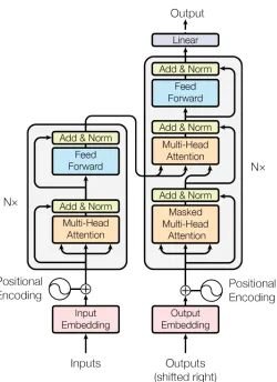
Vaswani et al. (49) introduced The Transformer to overcome the various drawbacks of
RNNs discussed above. The basic structure of the Transformer network, as shown in
figure 2.3 resembles a standard auto-encoder consisting of two networks which model
opposite transformations on data and the latent space. The encoder maps an input
se-quence of pose representations (x1, x2, ..., xS) to a sequence of continuous latent space
(z1, z2, ..., zS), wherext ∈IRd model; zt ∈IRd model; S is the sequence length; and d model
is the dimensionality on the model and is a hyper-parameter. The decoder produces an output sequence (y1, y2, ..., ys) conditioned on the latent code z.
This basic structure forms the core of the network which is augmented with
self-attention mechanism and feed-forward networks which make up the internal structure of
the encoder and decoder networks. To achieve a robust forecasting performance, multiple
blocks of these encoder and decoder networks are stacked on top each other creating
a layered model. Tuning this hyperparameter, N which defines the number of identical
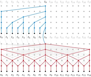
Figure 2.2: The ByteNet structure - the decoder (blue part) is dynamically unfolded so that it is conditioned on the representations of the input sequence produced upto the present step.
2.2.1
Encoder and Decoder
EncoderEach encoder stack is comprised of two sub-layers, namely, a Multi-Headed Self-Attention
Mechanism, and a simple position-wise fully connected feed-forward layer. Each
sub-layer has a residual connection inspired from the ground-breaking paper from Microsoft
(20), which is followed by a Layer Normalization operation to negate a change in the
distribution of the inputs to the neurons of a hidden layer.
Decoder
Decoder is similarly stacked N times with an additional sub-layer to the layers discussed
above. The third sub-layer attends to specific past time instances in the output of the encoder. Hence, for each output time step, the network is able to learn important time
instance in the input sequence.
learning a unity mapping for future time steps. To achieve this, a binary mask is used
for each time instance which prevents the decoder from attending to future instances.
Figure 2.3: The Transformer structure
2.2.2
Attention Mechanism
Attention mechanism has emerged as a fairly popular concept in deep learning in recent
years. First proposed by Larochelle and Hinton (32) and Denil et al. (11) for the image
gives importance to certain aspects of the input.
The standard attention mechanism works by assigning a weight vector αi to each
feature vector i of the hidden representation of the input data. The weight vector is
calculated using an attention functionfatt which depends on the type of attention
mech-anism implemented. This weigh vector, along with the input representation, at, is used
to calculate thecontext vector, usingφ(.) which defines what the model is looking at, or
the most relevant parts of the input as determined by the attention function.
ˆ
zt =φ({at},{αt}) (2.1)
The underlying concept of attention can be implemented primarily in two distinct
ways:
• Stochastic Hard Attention
• Deterministic Soft Attention
Stochastic Hard Attention
In determining the location where the model decides to focus attention while generating
tth time-step, a location variables
t,i is defined as an one-hot encoded variable which is set
to 1 if theith location (out of the past time steps upto current) is the one used to create
the current time symbol. Hence, by treating the attention locations as intermediate latent
variables, we can assign a multinoulli distribution parameterized by αi given by:
p(st,1 = 1|sj<t,a) =αt,i (2.2)
ˆ
zt =
X
i
st,iai (2.3)
Deterministic Soft Attention
The term ”soft” here refers to a smooth probability distribution over not just one, but
multiple correlated time-steps, which the model learns using a differentiable attention
functionfatt. The strength of correlation is reflected by the weight vectorαt which sums
to unity. In other words, the weight vector is a softmax over an attention function which in turn is conditioned on the input hidden representation.
αti =
exp(eti)
P
kexp(etk)
(2.5)
This weight vector can now be used to compute the context vector as follows:
Ep(st|a)[ˆzt] = X
i
αt,iai (2.6)
The Transformer implements a soft self-attention mechanism, inspired by Cheng et al.
(7) and Luong et al. (38), which relates different parts of a sequence in order to compute a representation of the same sequence. The intuition behind self-attention can be
summa-rized as a mapping between a query and a set ofkey-value pairs. From a Neural Turing
Machine’s(19) perspective, the query is the symbol (time-instance) which the model is
currently trying to generate. Thekeysandvalues are represent all the symbols that occur
in the past.
Scaled Dot-Product Attention
While Luong et al. (38) showed that self-attention can be of multiple flavours, where the
model learns the context vectorct by either attending toall the previous symbols (global
context), or learn to attend to a subset of these symbols (local context), with different
alignment functions, we, however, focus on implementing only the global dot-product
attention mechanism due to its simplicity and hardware constraints on implementing
more complicated functions. A comparative study on implementing other functions will
make for an interesting ablation study.
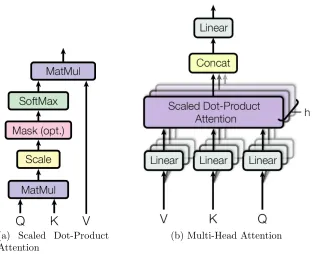
The ”Scaled Dot-Product Attention”, as shown in figure 4.6i consists of keys of
di-mension dk and values of dimension dv. We compute a dot-product of a query with all
the keys, and apply a softmax over the product. In practice, we scale the dot-product to prevent the softmax from saturating and hindering back-propagation due to vanishing
gradients. Figure ?? shows the attention block used here.
Attention(Q, K, V) = sof tmax(QK
T
√
dk
)V (2.7)
Multi-Headed Self-Attention
As we discussed earlier, a potential replacements for RNNs is the use of CNNs which are
(a) Scaled Dot-Product Attention
(b) Multi-Head Attention
Figure 2.4: Self-Attention mechanism structure
effective in extracting information from input data using multiple filter kernels. They
ac-complish this by transforming the input data using different linear projections to extract different information from the same input. This useful trait of a convolutional layer can
be leveraged by projecting the query and key-value pairs using different learned linear
projections. This forms the basis of multi-headed attention (figure 2.4b) where the model
learns to attend to different latent sub-spaces at different positions.
M ultiHead(Q, K, V) =Concat(head1, head2, ..., headh)WO
where headi =Attention(QW Q i , KW
K i , V W
V i )
(2.8)
In equation 2.8 the projection weights are parameter matrices WiQ ∈ IRdmodel×dk,
WK
i ∈IRdmodel
×dk, WV
i ∈ IRdmodel
×dv, WO ∈IRdhdv×dmodel. The number of heads h to
em-ploy, being a hyper-parameter, can be tuned to get interesting results which are discussed
in chapter 4.
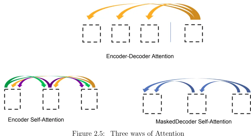
The Transformer uses three different modes of a soft self attention mechanism to learn long-term dependency as shown in figure 2.5. The encoder contains pure self
atten-tion mechanism where every symbol attends to every other symbol in the input sequence.
the entire input sequence. The decoder contains an attention block which maps encoded
input representation to each generated symbol. This enables the model to learn corre-lated positions in the input sequence to generate a new symbol at every time-step. For
generation, the model is not allowed to peek in the future, otherwise the model will tend
to learn a unity mapping between the ground-truth and the generated symbol, which
will hinder any inference capabilities once deployed. Hence it is important to prevent the
decoder from attending to future by using a masked attention scheme.
Figure 2.5: Three ways of Attention
2.2.3
Positional Embedding
Since the primary motivation of employing the Transformer is to remove dependency
on the sequential nature of RNNs, it becomes imperative that the model has a sense of temporal order in the input sequence, which is fed as a single 3-D tensor to the model.
One approach to achieve this is to add deterministic positional embeddings to the
input which are not learnt during training, but instead depend on the input positions.
This is a sustainable approach which scales well for longer sequence lengths and the
model remains flexible enough to accept different sequence lengths during testing.
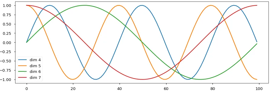
frequencies:
P E(pos,2i)=sin(pos/100002i/dmodel) P E(pos,2i+1)=cos(pos/100002i/dmodel)
(2.9)
On visual inspection of equation 2.9 in figure 2.6, it is clear that the embeddings
introduce a temporal order if added element-wise to the input tensor. The figure shows
the corresponding waveforms for dimensions 4 to 7 of the input feature space over a
possible 100 time-steps.
Figure 2.6: Positional Embeddings using sine and cosine waves.
2.2.4
Feed-Forward Network
Apart from the attention layers, each encoder and decoder block contains a fully con-nected feed-forward network which is applied separately and identically to each symbol
in the input to both encoder and decoder. This consists of two linear transformations
with a ReLU activation function between them. Each of these transformations is applied
to each symbol but with separate parameters to ensure separability across layers. The
dimensionality of the input and output of this network is dmodel and the inner dimension
is df f which is varied according to table 4.1.
2.2.5
Layer vs. Batch Normalization
The output of each sublayer in the encoder-decoder framework of the Transformer is
layer. This design choice stems from Lei Ba et al. (33) where they argue about the
demerits of batch normalization and introduce layer normalization as an alternative. Batch normalization(22) was introduced to reduce undesirable ”covariate shift”
be-tween the gradients of one layer and the outputs of the previous layer in a deep neural
network architecture. This change in parameters in a highly correlated structure causes
the network to converge slowly. To combat this, the summed inputs to each hidden unit
is normalized using the mean and standard deviation over all the training cases. This
puts an unreasonable amount of dependence on the batch size.
Layer normalization was introduced to reduce this dependence by calculating the
normalization statistics (mean and standard deviation) over all hidden units in a layer.
µl = 1
H
H
X
i=1 ali σl =
v u u t 1 H H X i=1
(ali−µl)
(2.10)
where, H is the number of hidden nuerons in a hidden layer l and al i = wli
T
hl is the
summed input to neuron i in layer l.
2.3
Variational Encoder
Traditional auto encoders can be visualized as comprised of two different networks; an
Encoder, which encodes the prior data distribution into a latent code, and a Decoder,
which tries to regenerate the data distribution given the latent code.
The latent code is a representation of the underlying data modalities that are effective
at explaining the complex data mani-fold. Learning a mapping between data and its latent
code is important to learn how it affects the data.
pθ(x) =
Z
pθ(x|z)pθ(z)dz (2.11)
As shown by 2.11, calculating the marginal likelihood of data consists of a prior,pθ(z),
over the latent code z, and the conditional probability pθ(x|z).
However, calculating the above integral is intractable due to the basic assumption that
2.12 also is intractable.
pθ(z|x) =
pθ(x|z)pθ(z)
pθ(x)
(2.12)
The primary goal of a generative model like a Variational Auto-Encoder (VAE) is to learn the true likelihood,pθ(x) of the data, which enables us to generate similar data
sam-ples from the learned distribution. However, due to the aforementioned intractability, we
estimate an approximation of the true posterior, called the variational posteriorqφ(z|x),
where φ are the parameters for learning this variational posterior which are learned by
the encoder.
In order to regenerate samples from this learned posterior, we sample zi ∼q
φ(z|xi).
This however, is not differentiable in a gradient based estimator. To tackle this problem
of high variance by vanilla gradient estimator, a reparametreization trick is presented in
(31).
Assuming the prior over the latent variable to be centered a isotropic multivariate
Gaussian distribution,pθ(z) =N(z; 0, I). Also,pθ(x|z) can be a multivariate Gaussian or
Bernoulli, parameters of which are computed from z using a neural network. Therefore,
the variational approximate posterior can be described as
qφ(z|x(i)) =N(z;µ(i), σ2(i)I) (2.13)
where µ(i) and σ(i) represent the mean and the standard deviation, respectively of the
approximate posterior, which are the outputs of the encoding network. The latent code
z(i) is sampled usingg
φ(x(i), (i)) =µ(i)+σ(i)·(i), where·shows the element-wise product
Chapter 3
Methodology
3.1
Problem Formulation
This work aims at focusing on the temporal nature of the problem, setting benchmarks
for future research. The algorithms/models are chosen because they have been widely
documented to be ideally suited for any kind of prediction problem. Hence they are employed here for a establishing baseline prediction performance for new, more complex
methods.
Concretely, these algorithms will try to predict pose points, which are represented
by 2-D coordinates of positions of specific joints of the human body in a d dimensional
vector for time step t. More formally, the input is represented as xt ∈ IRd. Given the
current time step t , we want to predict the values of x for j future time-steps when we
are given the data for the past n time steps. Therefore, we want:
E[xt+1:t+j] =f(xt−n:t;θ) (3.1)
where,θ are the parameters of the model which is defined by the prediction functionf(.)
The prediction function will depend on what model is being used. The primary model
being used here is the Transformer network which is compared to the baseline set by
a Recurrent Neural Network, specifically, the Long Short Term Memory (LSTM)(21)
3.2
Data
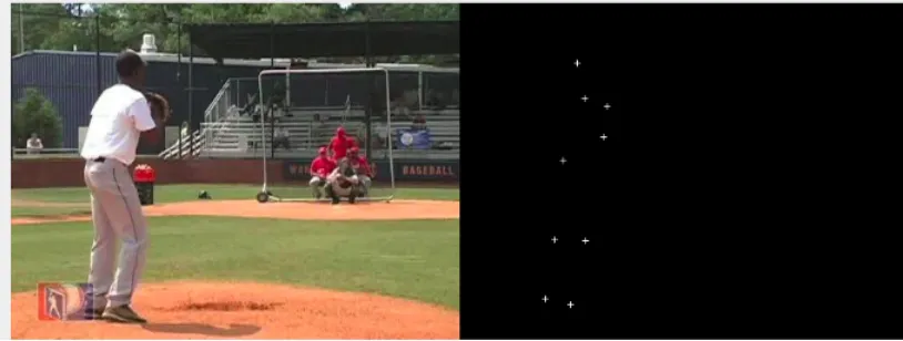
Here, Pose forecasting is evaluated in 2D using the Penn Action dataset(56). Penn Action
contains 2326 video sequences (1258 for training and 1068 for test) covering 15 sports
action categories. Each video frame is annotated with a human bounding box along with
the locations and visibility of 13 body joints. As shown in figure 3.1, the data contains
RGB images along with pose annotations.
Figure 3.1: Penn Action Dataset sample
MPII Human Pose dataset(Andriluka et al.) is a popular dataset to use for human
pose and gait analysis research. Like Penn Action, the dataset contains 2-D coordinates
of 16 key points of humans in the wild along with the bounding box coordinates. This
is a larger dataset than Penn Action by volume and size. However, the dataset contains
only three images in consecutive order, which limits its use for forecasting problems.
Another popular dataset used by many authors to test their pose forecasting models
is the Human3.6M(23)(5) dataset. This set contains 11 professional actors performing 17 different activities in a controlled laboratory environment. The human pose annotations
contain 3-D join positions and joint angles from a high-speed motion capture system.
Unlike, Penn Action, this contains human activity in an indoor environment performed
in a deliberate manner in a laboratory setting. This will introduce a bias in the model
which is supposed to capture the subtle and complex science of human gait in the wild.
Hence, this makes Human3.6M not ideal for this application.
re-cently (just over a month ago as evidenced by their GitHub commit history) released a
ground-breaking dataset PedX(29)(URL: http://pedx.io) which is ideal for human pose forecasting applied to forecasting pose for autonomous vehicles on busy and complex
intersections. The researchers even captured the data using a stationary autonomous car
parked on an intersection. The author notes that due to tight time constraints, this work
does not explore this beautiful dataset, which, however, makes for an interesting scope
for future work using Transformers.
As this is a temporal forecasting problem, we need to create sequences to be fed into
the LSTM model. These sequences are created using two different approaches: using a
strided sliding window and using a dilated sliding window, explained below. It is desirable
that the model is invariant to the starting frame, hence, we train the model with variable starting frames. Additionally, we fix a reasonable sequence length of 16 frames, where we
use frames 0 through 15 as the input sequence to predict frames 1 through 16.
3.2.1
Dilated Sliding Window
For a video sequence with K frames, we generate K sequences by varying the
start-ing frame. The dilated window effect is created by skippstart-ing frames when generatstart-ing
sequences. The number of frames skipped is video dependent. Therefore, for a video
con-taining K frames, we skip (K −1)/15 from the raw video sequence. This is to ensure
that a particular sequence is able to reach the end of the raw sequence and also to reduce
redundant information between adjacent frames. Once we go past the final frame of a
video sequence, we repeat the last collected frame until we obtain 16 frames.
However, this approach introduced high prediction variance for last few frames of a
sequence. The evaluation metrics for last frames of a sequence reduced considerably as
compared to the metrics for first few frames.
3.2.2
Strided Sliding Window
Here, we discard the idea of skipping frames because of high prediction variance. Instead,
we utilize a sliding window where we extract K contiguous frames from a raw video
sequence containing K frames by varying the starting frame. This results in a reduced
3.3
Experiments
3.3.1
Naive Pose Forecasting
To evaluate the Transformer model for pose forecasting, we train the model on raw human
skeleton data from Penn Action. The pose points are normalized according to the section
3.4 to make the model invariant to human position in the image - as described by the
2-D coordinates of the skeleton.
The model is trained to predict 8 frames in the future, given 8 past frames. Here, the
model is conditioned on frames which are described by raw pose points flattened into ad
dimensional vector as described in section 3.1. Therefore, each frame is represented by a
d= 2N dimensional vector, where N is the number of keypoints present in the dataset.
3.3.2
Pose Forecasting using Global Context
Forecasting human pose in future timesteps involves a complex manifold of human gait
and its multi-modal constraints as well as external factors which are not captured. These
external factors involve the immediate surroundings of a human subject, which
deter-mine the trajectory as well as speed of motion eventually observed. A human pedestrian
standing at a signal will not step onto the road if there are vehicles still moving around him. This global context information is needed to effectively forecast the next movement
of a human subject.
To achieve this, the global context information is added by approximating the
vari-ational posterior of the latent code of each RGB image frame using an 18-layer CNN
with residual connections - ResNet18(20). Each image is encoded into a dh dimensional
vector, which is then concatenated with the pose vector to form a d+dh dimensional
input vector for each frame.
3.4
Preprocessing
As the input data consists of the actual location of keypoints in the 2-D plane of an image,
normalizing the data is imperative to make the model invariant to the location of the
human subject in the frame. To achieve this, each 2-D keypoint is scaled by subtracting the centroid of a tight bounding box around a human subject and dividing the result by
the maximum dimension of this box. The tight bounding box is extracted by taking the
For training involving images, each image frame was first cropped using the given
bounding box parameters. Then, each image was resized to 256×256, while preserving the original aspect ratio of the image. This was done by calculating a scaling ratio between
the desired image size and the maximum of the original image dimensions. This ratio was
used to scale the other image dimension as well as the pose vector to maintain sanity.
3.5
Optimizer and Learning Rate Schedule
The optimizer used in this work is the Adam optimizer(30) withβ1 = 0.9,β2 = 0.98 and
= 109. The learning rate is varied according to the following formula:
lrate=d−0model.5 ·min(step num−0.5, step num·warmup steps−1.5) (3.2) Thus, the learning rate follows a additive-increase/multiplicative-decrease schedule
where the learning rate increases linearly for the first warmup steps training steps, and
decreases thereafter proportionally to the inverse square-root of the current training step
number.
3.6
Loss function and Evaluation Metric
The training loss function used is the Euclidean distance metric which is used to directly
minimize the distance between the predicted human pose vector for each frame with the
ground-truth pose vector.
While evaluating a model, this work adopts the standard Percentage of Correct
Key-points (PCK) metric introduced by (Andriluka et al.). PCK measures the accuracy of predicted keypoints by considering a predicted keypoint as correct if it lies within a
certain distance from the corresponding ground-truth point. This distance threshold is
typically based on the size of the full body bounding box. Here, the PCK distance
thresh-old is taken to be 0.05×max(h, w), whereh, ware the dimensions of the body bounding
box. PCK is computed for each of the predicted frames separately and averaged across
3.7
Hardware and Training Schedule
The models were trained using the PyTorch(40) deep learning framework. To have a
level comparison filed, all the models were trained using the optimizer and learning rate
schedule as described in section 3.5.
The training-testing split is used as provided by the dataset which resulted in 68672
training and 60277 testing sequences with a sequence length of 16. As mentioned earlier,
all models are trained to generate 8 frames conditioned on 8 past frames.
For naive pose forecasting, all models are trained with a batch size of 64 for 1073
training steps per epoch, for 6 epochs. The optimizer warmup steps of 2900 gave the most stable model.
When training with images, the hardware constrained the batch size to just 8 due to
the large image dimensions being loaded in the GPU memory. The models were trained
for 47890 training steps with the learning rate increasing for 15000 steps.
The models were trained on a single NVIDIA Tesla P100 with 16GB device memory.
The average training time for the naive transformer was around 8 hours as compared to
11.5 hours for the naive LSTM. For training with global image context, the training time
Chapter 4
Results
We report the performance of this novel neural network architecture, originally designed
for language translation, in effectively forecasting human pose. As described in section
3.3, the ablation study consists of two main experiments: (1) Naive Pose Forecasting,
and (2) Pose forecasting with Global Context. For the naive forecasting model, there
are several model configurations possible to pin-point which aspect of the network is
really important for performance gains; this makes up a second level of ablations. For
the experiment using global image context, due to hardware constraints, we are able to explore only two of these ablations.
As a baseline, the excellent and pioneering work done by Fragkiadaki et al. (16)
where they used a three layered LSTM network to forecast pose vectors in the future
time-steps. The model is trained on the same data from scratch using the same optimizer
and learning rate schedule used for the Transformer. Figure 4.1 shows the PCK and the
euclidean distance for forecasting 15 frames in the future given one single start frame.
The metrics are averaged over the entire test data for each predicted frame.
4.1
Ablations
4.1.1
Change in network structure
To evaluate the importance of different aspects of the model, we varied the base model by
changing different parameters and measuring the performance on the test data of Penn Action. Table 4.1 gives a summary of different model variations tested and evaluated on
the PCK metric. The table also shows PCK for the last predicted frame (that is, frame
In table 4.1, rows (A) show the models with different number of attention heads and
key-value dimensions. Contrary to a CNN where more number of filter kernels usually gives a better performance, here the model doesn’t perform as well as the best setting
even with more number of heads.
Table rows (B) show that increasing the model size, and consequently the number of
trainable parameters, improves the performance, although not always. Not surprisingly,
the best performance was given by the biggest model on the list.
The main selling point of the transformer is that even though the number of
param-eters is way more than the baseline LSTM model, none of the models took more than
10 hours to converge during training; the LSTM model took just more than 12 hours of
training time.
For evaluation, the trained models were given exactly one start frame and queried
to produce the next 15 frames conditioned on that one start frame. Table 4.2 shows a
subset of the performance achieved by each model. Additionally, figure 4.1 shows PCK
with the MSE forecasting metric.
Figures 4.3 and 4.4 show the performance comparison for short-term and long-term
forecasting for abaseball pitch, respectively. The top row in each image is the ground truth
Table 4.1: Model variations
N dmodel df f h dk dv Pdrop train
steps
[email protected] params (×106)
BASE 6 512 2048 8 64 64 0.1 6.4k 0.4615 44.18
(A)
1 512 512 0.6153
4 128 128 0.4615
16 32 32 0.5076
32 16 16 0.5239
(B)
2 0.6923 14.75
4 0.6153 29.47
8 0.5538 58.89
256 32 32 0.6 17.38
1024 128 128 0.7077 126.09
1024 0.4769 31.59
4096 0.5385 69.37
BIG 6 1024 4096 16 0.3 16k 0.8154 176.44
Table 4.2: Model ablation results
TX Frame #
Model Config. 1 5 7 13 14 15
BASE 1 0.7230 0.5384 0.4307 0.4615 0.4615 A1 1 0.9846 0.8461 0.6307 0.6153 0.6153
A2 1 0.5846 0.4153 0.4461 0.4615 0.4615 A3 1 0.9230 0.8461 0.5076 0.5076 0.5076 A4 1 0.8461 0.7692 0.6769 0.6461 0.5239 B1 1 1 0.9230 0.6923 0.6923 0.6923
B2 1 0.8769 0.7692 0.6307 0.6153 0.6153 B3 1 0.7384 0.6923 0.6153 0.5692 0.5538
B4 1 0.8461 0.7538 0.6 0.5846 0.6
pose skeleton. The middle row in each image is the output from the baseline LSTM-3LR
model with dropout percentage set at 0.1, whereas the last row in each image is the output from the BIG version of Transformer as detailed in table 4.1. The images clearly
show that the Transformer model is more adept at predicted in the immediate future,
while the LSTM model is better at long-term forecasting compared to the short-term.
The transformer also produced a smoother transition between frames as compared to the
jagged transition sequence from the LSTM.
Figures 4.5 and 4.6 show a failure case for short-term and long-term golf swing.
The transformer was unable to learn the multi-modal skeletal space, hence resulted in
outputting just one pose for the entire sequence.
4.1.2
With global image context
Human movement is often influenced by the dynamic environment surrounding the hu-man subject. Towards this effort, we introduce the global image context by encoding
the RGB image corresponding to each pose vector, which together describe a particular
frame. To encode this image, we use a standard ResNet18 network to approximately
estimate the variational posterior of our data. The encoded image is encoded into a
k−dimensional vector, which is concatenated with the corresponding pose vector,
re-sulting in a d = 26 +k dimensional vector which is input to the networks. Encoding
the image frames into a k= 5 dimensional vector gave us the best results from a search
space of 2,5,10,20 dimensions. Rest of the training schedule is identical to the naive
forecasting experiments, however, due to the added model complexity, and access to the same hardware and time constraints, we train the BASE Transformer model only. We
noticed there is indeed an improvement on the PCK metric (figure 4.2) due to the
en-coded image which empirically proves that the global context lends to an overall increase
in the forecasting performance. However, the performance when compared to the LSTM
baseline is not encouraging. We are still trying to gauge the viability of this solution as
Figure 4.2: Transformer(BASE) vs LSTM - test PCK and MSE using image context
(g) t=1 (h) t=5 (i) t=7
(g) t=13 (h) t=14 (i) t=15
Figure 4.4: Baseball Pitch long-term forecasting
(g) t=1 (h) t=5 (i) t=7
(g) t=13 (h) t=14 (i) t=15
Chapter 5
Conclusions
As mentioned earlier, pose forecasting seems an ideal application to exploit the highly
parallelizable architecture to improve training and inference time in a real-time
applica-tion. This work analytically proves that Transformers are better at maintaining long term
dependencies by better predicting the motion of a human subject performing complex
activities with varied posture. At their best, the Transformers improved on the current
baseline LSTM model by almost 5% with a vastly improved training time.
We note that a language model, at the time of writing this, hasn’t been previously used for a task outside its main domain like pose forecasting. This work not only encourages
a novel viewpoint to solve a complex sequence prediction task, but also motivates and
sets a bar for future research on this topic.
A deep dive into this problem has unearthed a slew of interesting and important
directions. The data used in evaluating Transformers is a relatively easy dataset where
the actions are well defined. A more challenging data would be PedX where the images
and pose captured are of actual pedestrians on a busy intersection.
Also, this system is aimed at improving self-driving path and motion planning, hence
the model needs to be trained on images and pose data through a dash-mounted camera. This poses several challenges and scaling the current system for achieving robust and
reliable inference is non-trivial. One of the major challenges that needs to be addressed
is the motion of the camera itself, which affects the 3-D joint locations with respect to
the camera.
As more money and research is poured into autonomous vehicles to perfect its
technol-ogy, this thesis serves as a small step forward for making autonomy a safer and sustainable
REFERENCES
[Andriluka et al.] Andriluka, M., Pishchulin, L., Gehler, P., and Schiele, B.
[2] Arjovsky, M., Chintala, S., and Bottou, L. (2017). Wasserstein gan. arXiv preprint arXiv:1701.07875.
[3] Bahdanau, D., Cho, K., and Bengio, Y. (2014). Neural machine translation by jointly learning to align and translate. arXiv preprint arXiv:1409.0473.
[4] Bissacco, A., Yang, M.-H., and Soatto, S. (2007). Fast human pose estimation us-ing appearance and motion via multi-dimensional boostus-ing regression. In 2007 IEEE conference on computer vision and pattern recognition, pages 1–8. IEEE.
[5] Catalin Ionescu, Fuxin Li, C. S. (2011). Latent structured models for human pose estimation. InInternational Conference on Computer Vision.
[6] Chen, Y., Shen, C., Wei, X.-S., Liu, L., and Yang, J. (2017). Adversarial posenet: A structure-aware convolutional network for human pose estimation. CoRR, abs/1705.00389, 2.
[7] Cheng, J., Dong, L., and Lapata, M. (2016). Long short-term memory-networks for machine reading. arXiv preprint arXiv:1601.06733.
[8] Chiu, C.-C., Sainath, T. N., Wu, Y., Prabhavalkar, R., Nguyen, P., Chen, Z., Kannan, A., Weiss, R. J., Rao, K., Gonina, E., et al. (2018). State-of-the-art speech recogni-tion with sequence-to-sequence models. In 2018 IEEE International Conference on Acoustics, Speech and Signal Processing (ICASSP), pages 4774–4778. IEEE.
[9] Chou, C.-J., Chien, J.-T., and Chen, H.-T. (2017). Self adversarial training for human pose estimation. arXiv preprint arXiv:1707.02439.
[10] Deng, J., Dong, W., Socher, R., Li, L.-J., Li, K., and Fei-Fei, L. (2009). ImageNet: A Large-Scale Hierarchical Image Database. In CVPR09.
[11] Denil, M., Bazzani, L., Larochelle, H., and de Freitas, N. (2012). Learning where to attend with deep architectures for image tracking. Neural computation, 24(8):2151– 2184.
[12] Devlin, J., Chang, M.-W., Lee, K., and Toutanova, K. (2018). Bert: Pre-training of deep bidirectional transformers for language understanding. arXiv preprint arXiv:1810.04805.
[13] Du, X., Vasudevan, R., and Johnson-Roberson, M. (2019). Bio-lstm: A biomechan-ically inspired recurrent neural network for 3-d pedestrian pose and gait prediction.
[14] Fang, H.-S., Xie, S., Tai, Y.-W., and Lu, C. (2017). Rmpe: Regional multi-person pose estimation. In Proceedings of the IEEE International Conference on Computer Vision, pages 2334–2343.
[15] Ferrucci, D., Brown, E., Chu-Carroll, J., Fan, J., Gondek, D., Kalyanpur, A. A., Lally, A., Murdock, J. W., Nyberg, E., Prager, J., et al. (2010). Building watson: An overview of the deepqa project. AI magazine, 31(3):59–79.
[16] Fragkiadaki, K., Levine, S., Felsen, P., and Malik, J. (2015). Recurrent network models for human dynamics. InProceedings of the IEEE International Conference on Computer Vision, pages 4346–4354.
[17] Gehring, J., Auli, M., Grangier, D., Yarats, D., and Dauphin, Y. N. (2017). Con-volutional sequence to sequence learning. In Proceedings of the 34th International Conference on Machine Learning-Volume 70, pages 1243–1252. JMLR. org.
[18] Goodfellow, I., Pouget-Abadie, J., Mirza, M., Xu, B., Warde-Farley, D., Ozair, S., Courville, A., and Bengio, Y. (2014). Generative adversarial nets. In Advances in neural information processing systems, pages 2672–2680.
[19] Graves, A., Wayne, G., and Danihelka, I. (2014). Neural turing machines. arXiv preprint arXiv:1410.5401.
[20] He, K., Zhang, X., Ren, S., and Sun, J. (2016). Deep residual learning for image recognition. In Proceedings of the IEEE conference on computer vision and pattern recognition, pages 770–778.
[21] Hochreiter, S. and Schmidhuber, J. (1997). Long short-term memory. Neural com-putation, 9(8):1735–1780.
[22] Ioffe, S. and Szegedy, C. (2015). Batch normalization: Accelerating deep network training by reducing internal covariate shift. arXiv preprint arXiv:1502.03167.
[23] Ionescu, C., Papava, D., Olaru, V., and Sminchisescu, C. (2014). Human3.6m: Large scale datasets and predictive methods for 3d human sensing in natural environments.
IEEE Transactions on Pattern Analysis and Machine Intelligence, 36(7):1325–1339.
[24] Jain, A., Tompson, J., Andriluka, M., Taylor, G. W., and Bregler, C. (2013). Learn-ing human pose estimation features with convolutional networks. arXiv preprint arXiv:1312.7302.
[25] Jain, A., Zamir, A. R., Savarese, S., and Saxena, A. (2016). Structural-rnn: Deep learning on spatio-temporal graphs. In Proceedings of the IEEE Conference on Com-puter Vision and Pattern Recognition, pages 5308–5317.
[27] Kalchbrenner, N., Espeholt, L., Simonyan, K., Oord, A. v. d., Graves, A., and Kavukcuoglu, K. (2016). Neural machine translation in linear time. arXiv preprint arXiv:1610.10099.
[28] Kendall, A., Grimes, M., and Cipolla, R. (2015). Posenet: A convolutional network for real-time 6-dof camera relocalization. In Proceedings of the IEEE international conference on computer vision, pages 2938–2946.
[29] Kim, W., Ramanagopal, M. S., Barto, C., Yu, M.-Y., Rosaen, K., Goumas, N., Vasudevan, R., and Johnson-Roberson, M. (2019). Pedx: Benchmark dataset for metric 3-d pose estimation of pedestrians in complex urban intersections. IEEE Robotics and Automation Letters, 4(2):1940–1947.
[30] Kingma, D. P. and Ba, J. (2014). Adam: A method for stochastic optimization.
arXiv preprint arXiv:1412.6980.
[31] Kingma, D. P. and Welling, M. (2013). Auto-encoding variational bayes. arXiv preprint arXiv:1312.6114.
[32] Larochelle, H. and Hinton, G. E. (2010). Learning to combine foveal glimpses with a third-order boltzmann machine. InAdvances in neural information processing systems, pages 1243–1251.
[33] Lei Ba, J., Kiros, J. R., and Hinton, G. E. (2016). Layer normalization. arXiv preprint arXiv:1607.06450.
[34] Liu, C., Liu, J., Huang, J., and Tang, X. (2010). Monocular video based marker-less 3d human pose estimation by using local multi-connected belief propagation with multi-cue fusion. In 2010 IEEE International Conference on Intelligent Computing and Intelligent Systems, volume 1, pages 478–482. IEEE.
[35] Liu, C.-G., Cheng, D.-S., Liu, J.-F., Huang, J.-H., and Tang, X.-L. (2011). Inter-active particle filter based algorithm for tracking multiple objects in videos. Dianzi Xuebao(Acta Electronica Sinica), 39(2):260–267.
[36] Lotter, W., Kreiman, G., and Cox, D. (2015). Unsupervised learning of visual struc-ture using predictive generative networks. arXiv preprint arXiv:1511.06380.
[37] Luo, Y., Ren, J., Wang, Z., Sun, W., Pan, J., Liu, J., Pang, J., and Lin, L. (2018). Lstm pose machines. InProceedings of the IEEE Conference on Computer Vision and Pattern Recognition, pages 5207–5215.
[38] Luong, M.-T., Pham, H., and Manning, C. D. (2015). Effective approaches to attention-based neural machine translation. arXiv preprint arXiv:1508.04025.
[40] Paszke, A., Gross, S., Chintala, S., Chanan, G., Yang, E., DeVito, Z., Lin, Z., Des-maison, A., Antiga, L., and Lerer, A. (2017). Automatic differentiation in pytorch.
[41] Pearson, K. (1895). Note on regression and inheritance in the case of two parents.
Proceedings of the Royal Society of London, 58:240–242.
[42] Saito, M., Matsumoto, E., and Saito, S. (2017). Temporal generative adversarial nets with singular value clipping. In IEEE International Conference on Computer Vision (ICCV), volume 2, page 5.
[43] Silver, D., Huang, A., Maddison, C. J., Guez, A., Sifre, L., Van Den Driessche, G., Schrittwieser, J., Antonoglou, I., Panneershelvam, V., Lanctot, M., et al. (2016). Mas-tering the game of go with deep neural networks and tree search.nature, 529(7587):484.
[44] Silver, D., Schrittwieser, J., Simonyan, K., Antonoglou, I., Huang, A., Guez, A., Hubert, T., Baker, L., Lai, M., Bolton, A., et al. (2017). Mastering the game of go without human knowledge. Nature, 550(7676):354.
[45] Toshev, A. and Szegedy, C. (2014). Deeppose: Human pose estimation via deep neural networks. InProceedings of the IEEE conference on computer vision and pattern recognition, pages 1653–1660.
[46] Toyer, S., Cherian, A., Han, T., and Gould, S. (2017). Human pose forecasting via deep markov models. In 2017 International Conference on Digital Image Computing: Techniques and Applications (DICTA), pages 1–8. IEEE.
[47] Van Den Oord, A., Dieleman, S., Zen, H., Simonyan, K., Vinyals, O., Graves, A., Kalchbrenner, N., Senior, A. W., and Kavukcuoglu, K. (2016). Wavenet: A generative model for raw audio. SSW, 125.
[48] Vaswani, A., Bengio, S., Brevdo, E., Chollet, F., Gomez, A. N., Gouws, S., Jones, L., Kaiser, L., Kalchbrenner, N., Parmar, N., et al. (2018). Tensor2tensor for neural machine translation. arXiv preprint arXiv:1803.07416.
[49] Vaswani, A., Shazeer, N., Parmar, N., Uszkoreit, J., Jones, L., Gomez, A. N., Kaiser, L., and Polosukhin, I. (2017). Attention is all you need. In Advances in Neural Information Processing Systems, pages 5998–6008.
[50] Vemula, A., Muelling, K., and Oh, J. (2018). Social attention: Modeling attention in human crowds. In2018 IEEE International Conference on Robotics and Automation (ICRA), pages 1–7. IEEE.
[52] Xiao, B., Wu, H., and Wei, Y. (2018). Simple baselines for human pose estimation and tracking. InProceedings of the European Conference on Computer Vision (ECCV), pages 466–481.
[53] Xu, K., Ba, J., Kiros, R., Cho, K., Courville, A., Salakhudinov, R., Zemel, R., and Bengio, Y. (2015). Show, attend and tell: Neural image caption generation with visual attention. InInternational conference on machine learning, pages 2048–2057.
[54] Xue, T., Wu, J., Bouman, K., and Freeman, B. (2016). Visual dynamics: Proba-bilistic future frame synthesis via cross convolutional networks. InAdvances in Neural Information Processing Systems, pages 91–99.
[55] Yoo, Y., Yun, S., Chang, H. J., Demiris, Y., and Choi, J. Y. (2017). Variational au-toencoded regression: high dimensional regression of visual data on complex manifold. InProceedings of the IEEE Conference on Computer Vision and Pattern Recognition, pages 3674–3683.