Small Secure Sketch for Point-Set Difference
Ee-Chien Chang Qiming Li
Department of Computer Science National University of Singapore
[email protected] [email protected]
Abstract. A secure sketch is a set of published data that can help to recover the original bio-metric data after they are corrupted by permissible noises, and by itself does not reveal much information about the original. Several constructions have been proposed for different metrics, and in particular, set difference. We observe that in many promising applications, set difference alone is insufficient to model the noises. We propose to look into point-set difference, which mea-sures noises that not only remove/introduce new feature points in the biometric objects, but may also perturb the points. In this paper, we first give an improvement for set difference construction that can be extended to multi-sets, where the sketch is small and there is an efficient decoding algorithm. We next give a sketch for point-set difference in both one and two-dimensional spaces. By using results in almostk-wise independence, the size of the sketch is reduced to near-optimal.
Keywords:biometrics, error-tolerant cryptography, secure sketch, point-set difference.
1 Introduction
Most biometric data are noisy in the sense that the capturing devices and extraction algorithms introduce inevitable noises. However, conventional cryptographic primitives do not tolerate even the slightest change in the data. For example, in an encryption scheme, decryption would fail if one bit of the decryption key is flipped. To use biometric data in cryptographic schemes (e.g., to use a fingerprint as the decryption key), new primitives are proposed (such as [9, 8, 6, 3]) to achieve robustness against noises. Secure sketch and fuzzy extractor were introduced in [6] as a generic way to reconstruct or extract a secret from noisy biometric data by publishing a “sketch”. Given a set of original biometric data X captured during the registration process, the encoder computes a sketch P and publishes it. Later, when a set of corrupted biometric dataY is presented, the decoder can recover the originalXfromP andY, as long asY is close toX under certain distance measure. The security is measured by the amount of information about X revealed by the sketch P. Since the distribution of X may not be uniform, fuzzy extractors perform an additional step on the reconstructed X to obtain a uniformly random key.
Although information leakage is the main concern, in some applications, it is desirable to have small sketches. For example,approximate message authentication codessuch as [11, 5] are developed to authenticate images under noises. Here, a short code is used to authenticate a long message received from a noisy channel. From another point of view, a small sketch simplifies the analysis of the information leakage, since the size of the sketch gives an upper bound of the information revealed.
the type of noises to be tolerated. Secure sketch schemes for the following two main types of biometric data have been proposed: (1) The biometric data are from a vector space, and the distance is measured using a norm, e.g., Hamming distance. (2) The biometric data X is a subset of a universeU, and the distance of two setsXandY, where|X|=|Y|=s, is measured by the set difference (s− |X∩Y|).
We observe that for many biometric feature representations, especially those involve images, a combination of the above is required. For example, a fingerprint is typically represented as a set of minutia, which are points in a 2-dimensional space [0,1]×[0,1], or even 3-dimensional if the less reliable orientation attribute is included [4]. The noises introduced during scanning usually lead to small perturbation of the minutia, together with removal and addition of minu-tia. Hence, it is common to model the noises as a combination of two types of noises. The first type of noise perturbs each point in X by at most a small distance, say δ, and we call this thewhite noise. Thereplacement noise replaces some points in the perturbedX by randomly selected points in U. The similarity between two setsX and Y can be measured by the max-imum number of pairs of matched points, where two points x and y are considered a match if the distance between x and y is at mostδ. Let us call this measure between two point-sets
point-set difference. The following are a few observations that lead to our construction.
0-1 noise. Let us illustrate an observation using point-set X from the one-dimensional interval [0, n], andδ = 1/2. To handle the white noise, prior to all operations, one may round each point to its nearest integer. Hence, if a pointxis corrupted by a white noise, its rounded value could be unchanged, increased by 1, or decreased by 1. Therefore, to consider point-set difference in the continuous domain [0, n], it suffices to consider points in Zn, whereby the
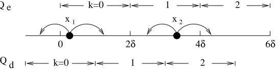
white noise either leaves each point unchanged, or increases/decreases it by 1. By using two different rounding algorithms during the encoding and the decoding, we can further assume that the white noise is 0-1, which either leaves each point unchanged, or increases it by 1 (Section 5). For a quick glance of why it is possible, refer to Fig. 1. Since it suffices to consider 0-1 noises, from now onward, we would only consider 0-1 noises in the discrete domain Zn.
To avoid the special case at the boundary, we assume that the0-1 noise has no effect on the point x=n−1.
Well-separation and multi-sets. Let us consider the pointsx3, x4andx5 in Fig. 2. Under the quantization as illustrated in the figure, these points will be quantized to the same value 6. In this example, if the noise onx5 happens to increase it by 1, then the quantized value would be different. To guarantee the consistency in the quantized values, we assume that the point-set
X is well-separated. That is, for any two points x1, x2 ∈X,|x1−x2|>1.
Such assumption is rather restrictive. In practice, it is difficult to ensure that all points are well-separated. If the input happens to contain 2 points that are the same, or close to each other, some mechanism is required. One method is to remove one of the points. However, this will lower the overall performance. We prefer another method which is to simply include both points. As we can see from Fig. 2, in certain cases, the quantized points will remain the same, hence the average performance potentially can be better than the first method. Section 6.3 discusses more on the practical issues and a way to reduce (but not eliminate) the 0-1 noise. More interestingly, in order to include repeated points, we need a sketch for set difference that can handle multi-sets (a multi-set is a set that may have repeated elements). Currently known constructions do not support multi-sets.
Another perspective of our construction. Here is another method that is unsatisfactory. The sketch includes a large point-setRsuch thatX ⊂R. During decoding, points inY are matched with the points in R. Next, the techniques for set difference are used to recover the replaced points. However, this method reveals too much information aboutX, and its performance de-pends on the underlying distribution ofX. For example, if the underlying distribution is likely to generate collinear points in X, then publishing R will reveal much about X. An improve-ment perturbs the points inX to obtainX0, and the sketch includes a point-setR0 such that
X0 ⊂R0. The setX is randomly perturbed so as to reduce the influence of the underlying dis-tribution. Although this approach seems feasible, there are many loose-ends. Our construction has many similarities with this approach, and indeed can be viewed as a method that realizes it.
In the rest of this paper, we first give a secure sketch for set difference that can handle multi-sets (Section 4). We then give a secure sketch for0-1noises for points in one-dimensional Zn(Section 6), and extend it to 2-dimensionalZn×Zn(Section 7). Although similar ideas can
be extended to higher dimensions, it might not be practical due to larger constant factors in the entropy loss.
Contributions and Results.
1. We give an approach to handle the combination of0-1noises and replacement noises, where the points are from a finite field Zn, and are well-separated. The total size of the sketch
2. We give an extension of the above to a 2-dimensional universe,Zn×Zn. If the encoder and
the decoder have polynomial computing time (with respect to s, t,logn), the entropy loss is at most 4s+ 4 + 2t(1 + 2 logn), while the size of the sketch is in O(slogn). When the encoder can do exhaustive search in 2Ω(s), then both the size of the sketch and the entropy loss are in O(s+tlogn).
3. We give a scheme for set difference that handles multi-sets. The scheme has a simple and yet very efficient decoding algorithm, which amounts to solving linear systems with 2t
equations, and root-finding for a polynomial of degree at most t. Hence, the number of arithmetic operations in Zn is bounded by a polynomial ofsand t. The size of the sketch
and the entropy loss are at most 2t(1 + logn). This construction is very similar to the set reconciliation technique in [10].
2 Related Works
Recently, a few new cryptographic primitives for noisy inputs are proposed. Fuzzy commitment scheme [9] is one of the earliest formal approaches to error tolerance. The fuzzy commitment scheme uses an error correcting code to handle Hamming distance. The notions ofsecure sketch
and fuzzy extractorare introduced in [6], which gives constructions for Hamming distance, set difference, and edit distance. Under their framework, a reliable key is extracted from noisy data by reconstructing the original data with a given sketch, and then applying a normal extractor (such as pair-wise independent hash functions) on the data. The issue ofreusabilityof sketches is addressed in [3]. It is shown that a sketch scheme that is provably secure may be insecure when multiple sketches of the same biometric data are obtained.
The set difference metric is first considered in [8], which gives afuzzy vault scheme. Later, [6] proposed three constructions. The entropy loss by all these schemes are roughly the same. They differ in the sizes of the sketches, decoding efficiency and also the degree of ease in prac-tical implementation. The BCH-based scheme [6] has small sketches and achieves “sublinear” (with respect to n, the size of the universe) decoding by careful reworking of the standard BCH decoding algorithm. All these schemes can not handle multi-sets. The set reconciliation protocol presented in [10] is designed for two parties to jointly discover the union of their data, with as little communication cost as possible. Although the problem settings are different, the techniques in handling set difference is similar and can be employed to obtain a secure sketch.
Another line of research yields the constructions of approximate message authentication codes([7, 2, 11, 5]), which can authenticate images that are corrupted by certain levels of noises, which are common to images (such as white noise and compression). There are also attempts in refining the extraction of biometric features so that the features are invariant to permissible noises [12]. Unfortunately, the reliability of such systems is not high.
3 Preliminaries
Entropy. Let H∞(A) be the min-entropy of random variable A, i.e., H∞(A) =
−log(maxaPr[A = a]). For two random variables A and B, the average min-entropy of A
given B is defined asHe∞(A|B) =−log(Eb←B[2−H∞(A|B=b)]). This definition is useful in the
analysis, since for any`-bit stringB, we haveHe∞(A|B)≥H∞(A)−`.
Secure sketch. LetMbe a set with acloseness relationC⊆ M × M. When (X, Y)∈C, we say theY is close toX, or (X, Y) is a close pair. The closeness can be determined by a distance functiondist:M × M →R≥0 and a threshold ∆. That is, (X, Y)∈Ciff dist(X, Y)≤∆.
Definition 1. A sketch scheme is a tuple (M,C,Enc,Dec), where Enc : M → {0,1}∗ is an encoder andDec:M × {0,1}∗ → Mis a decoder such that for all X, Y ∈ M,
Dec(Y,Enc(X)) =X, if (X, Y)∈C.
The string P =Enc(X) is to be made public and we call it the sketch. We say that the sketch
scheme ism-secure if for all random variableX over M, the entropy loss of P is at most m. That is, H∞(X)−He∞(X|Enc(X))≤m.
Closeness and Distance Functions. In this paper, M could be the collection of subsets or multi-sets of a universeU. The universe could beZnorZn×Zn, wherenis a prime. We consider
2 types of noises. The0-1noise, and the replacement noise that replaces certain elements in a set by randomly chosen elements. Here is a list of closeness and distance functions considered in this paper.
1. Cs,t: The closeness determined by set difference, which is catered for the replacement noise.
A pair (X, Y)∈Cs,t if|X|=|Y|=s and|X∩Y| ≥s−t.
2. ZDist: Distance function defined in Zn, which is catered for the 0-1noise.
ZDist(x, y) =
½
0 ify=x∨y=x+ 1
∞ otherwise . (1)
We defineZDist(n−1,0) =∞. We can generalize this function to 2 or higher dimensions. For example, inZn×Zn, we have
ZDist((x1, x2),(y1, y2)) =
½
0 ifZDist(x1, y1) = 0∧ZDist(x2, y2) = 0
∞ otherwise . (2)
Note thatZDistis not symmetric, that is, it is not necessary thatZDist(x, y) =ZDist(y, x). 3. ZPSs,t: Closeness for point-sets of size s. Suppose X = {x1, . . . , xs} and Y = {y1, . . . , ys},
we have (X, Y)∈ZPSs,t if there exists a 1-1 correspondencef on{1, . . . , s}such that
|{i|ZDist(xf(i), yi) = 0}| ≥s−t.
Almostk-wise independent random variables. A sample space onn-bit strings isk-wise inde-pendent if, the probability distribution, induced on everykbit locations in a randomly chosen string from the sample space, is uniform. Alon et al [1] considered almostk-wise independence with small sample size, and gave several constructions.
Definition 2 (Almost k-wise independence [1]). Let Sn be a sample space and X =
x1· · ·xn be chosen uniformly from Sn. Sn is almost k-wise independent with ² statistical
dif-ference if, for any k positions i1< i2 < . . . < ik, and any k-bit string α, we have X
α∈{0,1}k
|Pr[xi1xi2. . . xik =α]−2
−k| ≤². (3)
If we choose ²= 2−k, the probability Pr[xi
1xi2. . . xik = α] in (3) is non-zero. To see this, let
X0 =xi
1xi2. . . xik, then Pr[X
0 =α] = 0, and there exists some β 6=α such that Pr[X0 =β]>
2−k, since otherwiseP
α∈{0,1}kPr[X0 =α]<1. Thus|Pr[X0=α]−2−k|+|Pr[X0 =β]−2−k|>
2−k, which is a contradiction. Hence, we can always find suchX given any i
1, . . . , ik and any
α. Furthermore, the number of bits required to describe the sample is (2 +o(1))(log logn+ 3k/2 + logk) which is in O(k+ log logn).
4 Secure Sketch for Set Difference
In this section, we give a secure sketch for set difference, that is, with respect to the closeness Cs,t. Our scheme can handle the case where X is a multi-set. The size of the sketch is at most
2t(1 + logn). In addition, there exists a simple and yet efficient decoding algorithm – we just need to solve a linear system with 2tequations and unknowns and find the roots of two degree
tpolynomials.
To handle a special case, we assume thatXdoes not contain any element in{0,1, . . . ,2t−1}, and will discuss how to remove this assumption later at the end of this section. Our construction is similar to the set reconciliation protocol in [10], but the problem settings are different.
The encoder Encs. GivenX ={x1, . . . , xs}, the encoder does the following.
1. Construct a monic polynomial p(x) =Qsi=1(x−xi) of degree s. 2. Publish P =hp(0), p(1), . . . , p(2t−1)i.
The decoder Decs. Given P =hp(0), p(1), . . . , p(2t−1)i and Y ={y1, . . . , ys}, the decoder follows the steps below.
1. Construct a polynomial q(x) =Qsi=1(x−yi) of degree s. 2. Compute q(0), q(1), . . . , q(2t−1).
3. Let p0(x) =xt+Ptj−=01ajxj and q0(x) =xt+Ptj−=01bjxj be monic polynomials of degree t. Construct the following system of linear equations with the aj’s andbj’s as unknowns.
4. Find one solution for the above linear system. Since there are 2tequations and 2tunknowns, such a solution always exists.
5. Solve for the roots of the polynomials p0(x) andq0(x). Let them beX0 andY0 respectively.
6. Output Xe = (Y ∪X0)\Y0.
The correctness of this scheme is straight forward. When there is exactly t replacement errors, we can viewp0(x) as the “missed” polynomial whose roots are inX0=X\Y. Similarly,
q0(x) is the “wrong” polynomial, whose roots are in Y0 =Y \X. Since the roots of p(x) and
q(x) are inXand Y respectively, we have q(x)p0(x) =p(x)q0(x). This interpretation motivates the equation (4).
When there are less thantreplacement errors, there will be many degreetmonic polynomi-als p0(x) andq0(x) that satisfyq(x)p0(x) =p(x)q0(x). For any suchp0(x) andq0(x), they share
some common roots, which could be some arbitrary multi-set Z. That is, X0 = (X\Y)∪Z, and Y0 = (Y \X)∪Z. In Step 6, this extraZ will be eliminated.
When X∩ {0, . . . ,2t−1} 6= ∅, some equations in (4) would degenerate, which makes the rank of the linear system less than 2t. In this case, it is not clear how to find the correct polynomial in the solution space. Hence we require thatX∩ {0, . . . ,2t−1}=∅.
Note that in the above we do not require the elements of X and Y to be distinct, so this scheme can handle multi-sets. Furthermore, since the size of eachp(i) for 1≤i≤2t is (logn), the size of P is 2t(logn). Therefore, we have the
Lemma 1. WhenX∩ {0, . . . ,2t−1}=∅, the entropy loss due to Encs(X) is at most2tlogn.
Removing the assumption onX and Y. The assumption thatX cannot contain any element from{0, . . . ,2t−1}can be easily relaxed. We can find the smallest primemsuch thatm−n≥2t, and then apply the scheme on Zm. But instead of publishing p(0), . . . , p(2t−1), we publish p(m−1), . . . , p(m−2t). In this way, the size of the sketch is 2tlogm. In practice, this is not a problem since the size of the universe may not be prime, and we will need to choose a larger finite field anyway. For t that is not too large (say, t ≤n/4), we can always find at least one prime in [n+ 2t,2n]. Hence, we have the
Lemma 2. When t≤n/4, the entropy loss due to Encs(X) is at most 2t(1 + logn).
5 Reduction from White Noise to 0-1 Noise
Now we describe how to reduce the problem of dealing with white noises in a continuous domain to0-1noises in a discrete domain.
First, let us consider points in R, and the white noise that corrupts each point by at most
x∈[2kδ,2(k+1)δ). During decoding, we defineQd(y) =kif and only ify∈[(2k−1)δ,(2k+1)δ). Note that when|x−y| ≤δ, we haveQd(y)∈ {Qe(x), Qe(x) + 1}, hence the noise becomes0-1.
Therefore, instead of working with points from Rand white noises in the range [−δ, δ], it suffices to consider 0-1noises in Z. To avoid the special case at the boundary when working in the finite field Zn, we assume that the white noise has no effect on the last elementn−1.
0 2δ 4δ 6δ
x2 x1
Qd
Q e k=0 1 2
1 2
k=0
Fig. 1.Reduction from white noise to0-1noise.
6 0-1 Noise with Replacement when M= P(Zn)
In this section, we consider 0-1noise with replacement (the closeness ZPSs,t). The universe is
the one-dimensionalZn. We assume that the original biometric dataX is well-separated.
The final sketch published is a concatenation of two sketches, PHPS. The role of PH is to correct the0-1noise (Section 6.1 and 6.2).PH is the description of a quantizerH, whereby the quantized X remain the same under the0-1 noise. Since the quantized points are consistent, we can apply the techniques on set difference on them to correct the replacement noise. The sketch for set difference is PS. In this section, we focus on the construction ofPH.
6.1 Main Idea in Construction of PH
We render the elements inZn using two colors, black and white. For any x∈Zn,
color(x) =
½
white ifx≡1 mod 2
black ifx≡0 mod 2 (5)
We call a many-to-one function H a quantizer if for all x, H(x) = x if x is black, and H(x) is eitherx−1 or x+ 1 ifx is white. Fig. 2 depicts such a function. ForX ={x1, . . . , xs}, we denote H(X),{H(x1), . . . , H(xs)}.
Given X ={x1, x2, . . . , xs}, our goal is to find a quantizer such that each point in X will be consistently quantized, even under the influence of0-1noises. In particular, we require that
1 2 3 5 6
0 4 7 8
1
X X2 X4 X5
3 X
Fig. 2.A quantizerH. The arrows indicate how the points are quantized (or rounded) to even numbers.
H(x) H(x) H(x)
b b
b
(b) (c)
(a)
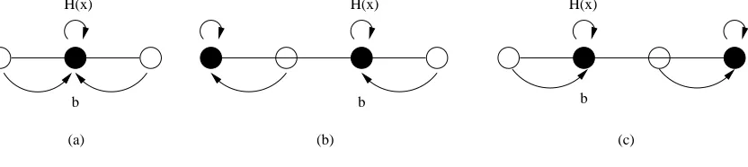
Fig. 3.RecoveringxfromH(x). There are three scenarios forH whenH(x) =b.
To reconstruct X given H(X), we need to add more constraints on H. Suppose we know that H(x) = b for some b, as illustrated in Fig. 3. In scenario (b) and (c), x must be b and
b−1 respectively. However, when (a) happens,x can be either borb−1.
To resolve the ambiguity, we addone but not both of the following two constraints:
§2a ∀x∈X, H(x+ 2) =x+ 3 ifx is white, or §2b ∀x∈X, H(x−1) =x−2 ifx is black.
Note that the constraint will not eliminate scenario (a). Nevertheless, even if scenario (a) happens, we can conclude that x=bif§2ais imposed, and thatx=b−1 if §2b is imposed.
6.2 Short Descriptions of H (Sketch PH)
A quantizer H can be conveniently represented by a sequence hh1, h3, h5, . . . , hn−2i where
hi = 0 ifH(i) =i−1; otherwise, hi = 1. Publishing such a sequence requiresbn/2cbits, which is undesirable when nis large.
For any given X, there would be many quantizers that satisfy the constraints in Section 6.1. The constraints restrict the values ofhi for certain indicesi’s. Let W be the set of these indices. For any otherj 6∈W,hj can be either 0 or 1.
The first constraint§1 restrictssof suchhi’s. For constraints§2aand§2b, we choose§2aif
We give two constructions of short descriptions. The first one is simple and efficient but requires |W|logn bits. The second one requires space that is near-optimal, but it requires exhaustive search during encoding. In either case, the entropy loss is small, and there exists efficient decoding algorithms. Letk=|W|, andW ={w1, . . . , wk}.
Construction I: Construct a polynomialf(x) of degreek−1 as the following.
1. Randomly choose d1, . . . , dk∈ U such that for 1≤i≤k,di ≡hwi mod 2.
2. Find a degree k−1 polynomialf such that f(wi) =di for 1≤i≤k.
The sketchPH is thekcoefficients off. Hence, the size of the sketch isklogn. The size of this sketch could be reduced further to aboutklog(n/2), since we can work on a smaller finite field. This is possible because the number of hi’s is only bn/2c, thus any finite field of size greater
thann/2 is sufficient.
During decoding, the quantizer H to be used is the one represented by hi = f(i) mod 2 for all oddi.
Construction II: Firstly we construct an almost k-wise independent space on n bits [1], and ²= 2−k. Given W and hhw1, . . . , hwki, we uniformly choose a sample β =β1· · ·βn in the
sample space such that βwi =hwi for alli. The representation ofβ is then the description of
H, which is the sketchPH. Note that the size of PH is`= (2 +o(1))(log logn+ 3k/2 + logk),
which is in O(s+ log logn). However, we do not have an efficient way to find such sample, except by exhaustive search in the sample space of size 2`. Nevertheless, the decoding can be
done efficiently.
Lemma 3. The entropy loss due to PH is at most 1.5s+ 1 for Construction I, and at most
(2 +o(1))(log logn+ 9s/4 + log(1.5s)) + 1, which is inO(s+ log logn), for Construction II.
Proof: For Construction I, we count the entropy. Let R be the randomness we invest in choosing the random numbers di’s. The entropy of R is k(logn−1) bits. The number of possible output of f is nk. Together with the one additional bit to choose the constraint, the
average min-entropy (X, R) given PH is at least He∞(X)−k−1. The randomness R can be
recovered fromX and PH. Therefore,He∞(X)−He∞(X|PH)≤k+ 1.
For Construction II, the entropy loss is simply bounded by the size ofPH. That is,He∞(X)−
e
H∞(X|PH)≤ |PH| ≤(2 +o(1))(log logn+ 3k/2 + logk) + 1.
Since k≤1.5s, we have the claimed bounds.
Recall from Section 4 thatPSintroduces entropy loss at most 2t(1+logn), the total entropy
loss of PHPS is bounded by the following.
6.3 On the Assumption that Points are Well-Separated
If the points are not well-separated, the error tolerance of our scheme would be affected. For example, consider the points x3, x4 and x5 in Fig. 2. If the 0-1 noise shifts x5 from 7 to 8, it will be considered as a replacement error. If the noise happens to leave x5 unchanged, then the scheme still works. In addition, ifX contains duplicated elements, our scheme would work fine because the sketch in Section 4 can handle multi-sets. In other words, our scheme has a guaranteed error tolerance when there are no two pointsx, x0 ∈X such thatx−x0= 1.
During the reduction from white noise to 0-1 noise as in Section 5, we can choose a step size that is larger than 2δ, such that given the same white noise, the points are less likely to be shifted. In other words, the 0-1 white noise is reduced on average. Note that this introduces more entropy loss. Moreover, such trade-off depends on the distribution of the input biometric data. Therefore, we will not discuss it further in this paper.
In sum, with the requirement on well-separation, our scheme can tolerate the claimed noise in the worst case. Without the requirement, the scheme could still perform well in average. Hence, it is better to include those points that violate the well-separation requirement, instead of removing them. To include those points, we have to handle multi-sets.
7 0-1 Noise with Replacement when M= P(Zn×Zn)
We now extend our construction on 0-1 noise with replacement to U = (Zn×Zn). Similar
to one-dimension, the sketch is the concatenated PHfPSf. We will only discuss the sketch PHf. We assume that X is always well-separated. That is, for any distinct (u1, v1),(u2, v2) ∈ X, |u1−u2| ≥2 and|v1−v2| ≥2.
7.1 Quantizer H
The elements in U are rendered with 4 different colors as below.
color(u, v) =
black ifu≡v≡0 mod 2
white ifu≡0 mod 2∧v≡1 mod 2 red ifu≡1 mod 2∧v≡0 mod 2 green ifu≡v≡1 mod 2
(6)
The0-1noise either leaves a pointxuntouched, or shifts it to one of the 3 adjacent points. Let Neighbour(u, v) be the set of 4 points that (u, v) may be shifted to by the 0-1 noise, namely {(u, v),(u+ 1, v),(u, v+ 1),(u+ 1, v+ 1)}.
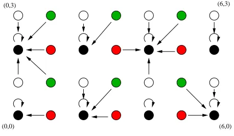
InZn×Zn, a quantizerH maps each point (u, v) to a black point (u0, v0) where|u−u0| ≤1
and |v−v0| ≤1. Fig. 4 illustrates such a quantizer. We need anH that satisfies the following:
For each (u, v) ∈ X, all the 4 points in Neighbour(u, v) are mapped to the black point in Neighbour(u, v). In other words,
(6,0) (6,3) (0,3)
(0,0)
Fig. 4.QuantizerH in 2-D.
In this way, if x∈X and y is a copy of x corrupted by0-1 noise, thenH(x) =H(y).
For each white and red point, there are two possible black points that it can be mapped to. It seems at first that there are four choices for each green point, but after the quantization for red and white points are fixed, only two choices are left. For instance, in Fig. 4, from the surrounding white and red points, we can deduce that the green point (3,1) can only be mapped to either (2,0) or (4,2). Hence, a straight forward description ofHrequires (1/4+1/4+1/4)n2 = (3/4)n2
bits.
We could apply similar ideas as in Section 6.2 to these (3/4)n2 bits to obtainPf
H. However,
there are still ambiguities to resolve when we recover X from H(X). For example, if H(x) = (0,2) as in Fig. 4, we would not be able to tell whetherx= (0,1) orx= (0,2). Our basic idea is to apply the ambiguity resolving techniques in Section 6.1 by imposing more constraints on
H. The details of the construction of PHf can be found in Appendix B.
Similar to 1-D, to obtain a short descriptionH, we identify the number of bits that have to be fixed due to the imposed constraints. In total, 3sbits are imposed by]1, and an additionals
bits are imposed by the constraints that resolve ambiguities. Then we can apply the techniques in Section 6.2. For instance, using Construction I as in the case of 1-D, we need to find a degree 4s−1 polynomial, which gives entropy loss at most 4s. We also need 4 additional bits to specify which color are the majority and minority in X. Thus, we have the following results.
Lemma 4. The entropy loss due toPfH is at most4s+ 4 with Construction I, and(2 +o(1))
(log(2 logn) + 6s+ log(4s)) + 4, which is inO(s+ log logn), with Construction II.
Theorem 2. When t≤ n2/4, the entropy loss due to PHf and PSf is at most h+ 4 + 2t(1 + 2 logn), whereh= 4sifPHf is computed using Construction I, andh= (2+o(1))(log(2 logn)+ 6s+ log(4s)) with Construction II.
References
2. G.R. Arce, L. Xie, and R.F. Graveman. Approximate image authentication codes. InProc. 4th Annual Fedlab Symp. on Advanced Telecommunications/Information Distribution, 2000.
3. Xavier Boyen. Reusable cryptographic fuzzy extractors. InProceedings of the 11th ACM conference on Computer and Communications Security, pages 82–91. ACM Press, 2004.
4. Michael D.Garris and R.Michael McCabe. Fingerprint minutiae from latent and matching tenprint images.
NIST Special Database 27, 2000.
5. G. DiCrescenzo, R. Graveman, G. Arce, and R. Ge. A formal security analysis of approximate message authentication codes. InProc. CTA Comm. and Networks, 2003.
6. Yevgeniy Dodis, Leonid Reyzin, and Adam Smith. Fuzzy extractors: How to generate strong keys from biometrics and other noisy data. InEurocrypt’04, volume 3027 ofLNCS, pages 523–540. Springer-Verlag, 2004.
7. R. Graveman and K. Fu. Approximate message authentication codes. InProc. 3rd Annual Fedlab Symp. on Advanced Telecommunications/Information Distribution, 1999.
8. Ari Juels and Madhu Sudan. A fuzzy vault scheme. InIEEE Intl. Symp. on Information Theory, 2002. 9. Ari Juels and Martin Wattenberg. A fuzzy commitment scheme. InProc. ACM Conf. on Computer and
Communications Security, pages 28–36, 1999.
10. Yaron Minsky, Ari Trachtenberg, and Richard Zippel. Set reconciliation with nearly optimal communications complexity. InISIT, 2001.
11. L. Xie, G.R. Arce, and R.F. Graveman. Approximate image message authentication codes. InIEEE Trans. on Multimedia, pages 242–252, 2001.
12. W. Zhang, Y.-J. Chang, and T. Chen. Optimal thresholding for key generation based on biometrics. Int. Conf. on Image Processing, 2004.
A Summary of Notations
n An odd prime.
U The universe, which could be Zn,Zn×Zn, or an Euclidean space.
M The set of biometric data. It is associated with a closeness relation.
X The original biometric data. X={x1, . . . , xs} ∈ M.
Y A copy of X corrupted by noise. Y ={y1, . . . , ys} ∈ M.
s The size of the biometric data X.
t The number of errors (w.r.t. to replacement noise) the scheme is designed to tolerate.
δ The amount of error (w.r.t. to white noise) the scheme is to tolerate.
P A sketch.
H A quantizer that handles 0-1noise.
H∞ Entropy. H∞(A) is the min-entropy of random variable A: H∞(A) =−log(maxaPr[A = a]).He∞(A|B) is the average min-entropy ofAgivenB:He∞(A|B) =−log(Eb←B[2−H∞(A|B=b)]).
Cs,t The closeness relation defined by set difference. A pair (X, Y) ∈Cs,t if|X|=|Y|=sand
|X∩Y| ≥s−t.
ZDist Distance function defined in Zn, which caters for the0-1noise. For x, y∈Zn,ZDist(x, y)
is defined to be 0 if 0≤y−x≤1, infinity otherwise.
B Detailed Construction of gPH
The quantizer H can be defined in terms of 3 functionsHw, Hr, and Hg,
H(x) =
Hw(x), ifcolor(x) =white Hr(x), ifcolor(x) =red Hg(x), ifcolor(x) =green
Each function maps its input to one of its neighbouring black points. For convenience, for any x ∈ X, let xb, xw, xr, and xg be the black, white, red and green points in Neighbour(x)
respectively. Hence, the first constraint]1 is equivalent to the following. For all x∈X,
]1a Hb(x) =xb ]1b Hw(x) =xb ]1c Hr(x) =xb ]1d Hg(x) =xb.
As mentioned in Section 7, there are two possibilities for Hr(x) and Hw(x), and once
they are fixed, there are also two possibilities for Hg(x). Hence, to describe H in a straight
forward manner using a binary sequence, we only need m = (1/4 + 1/4 + 1/4)n2 bits. Let
h=hh1, . . . , hmi be such a sequence.
For any x ∈X, to satisfy constraint ]1b, we need to restrict the value of at most one bit inh. Same for]1cand ]1d. We do not need to consider ]1a since it is implicit. Therefore, for
spoints, we need to restrict 3sbits inh.
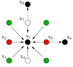
Similar to the 1-dimensional case, there will be ambiguities when we try to recover Xfrom anH that satisfies only ]1. One of the worst (most ambiguous) scenarios ofH is as illustrated by the solid arrows in Fig. 5. In this case, ifH(x) =x1 for somex∈X, any of the four points
X1
X4 X3
X2
X7 X8
X5 X6
Fig. 5.Ambiguity resolving in 2-D. The solid arrows show howHquantizes each point, and the dashed arrows show how the ambiguities can be resolved.
x1,x2,x3 and x4 could bex.
loss of generality, we assume that they are black and green respectively. Then we require that the following constraints are satisfied by H. For all (u, v)∈X,
]2a Hr(u+ 2, v) = (u+ 3, v) if (u, v) is red; ]2b Hw(u, v+ 2) = (u, v+ 3) if (u, v) is white; ]2c Both ]2aand ]2b if (u, v) is green.
With the above additional constraint, we can resolve the ambiguity by the following rules. If H is as shown by the solid arrows in the figure, we declare that x = x1. If Hr(x5) = x6 (the horizontal dashed arrow), and the rest follow solid arrows, we declare that x = x2. If
Hw(x7) = x8 (the vertical dashed arrow), and the rest follow solid arrows, we declare that
x=x4. If bothHr(x5) =x6 and Hw(x7) =x8, we declare thatx=x3.
In this case, each red and white point would restrict one more bit by constraints]2aand]2b
respectively, and each green point would restrict two more bits by constraint ]2c. Since green is the least frequently occurred color, the number of green points is at mosts/4. Similarly, the number of black points is at least s/4. In the worst case (in terms of the number of restricted bits), there ares/4 green points and s/2 red and white points. Therefore, the total number of bits restricted by these constraints is at most (1/2 + 2/4)s=s.