c
�Owned by the authors, published by EDP Sciences, 2018
General discussion on g-2
Marc Knecht1,a
1Centre de Physique Théorique, CNRS/Aix-Marseille Univ./Univ. du Sud Toulon-Var (UMR 7332) CNRS-Luminy Case 907, 13288 Marseille Cedex 9, France
Abstract.Progress made on the theoretical aspects of the standard model contributions to the anomalous mag-netic moment of the charged leptons since the first FCCP Workshop on Capri in 2015 is reviewed. Emphasis is in particular given to the various cross-checks that have already become available, or might become available in the future, for several important contributions.
1 Introduction
The anomalous magnetic moments of the electron (ae) and
of the muon (aµ) are among the most precisely measured quantities in particle physics. The latest available experi-mental results [1–3] read
aexpe = 1159652180.91(0.26)·10−12 [0.28ppb],
(1) aexpµ = 11 659 208.9(6.3)·10−10 [0.54ppm].
These measurements therefore represent stringent tests of the standard model, and constitute indirect windows to-wards possible degrees of freedom beyond it. Actually, due to the muon’s larger mass, its anomalous magnetic moment is expected to be more sensitive to new physics than the electron’s by a factor of (mµ/me)2 ∼ 4·104 [in
a strict sense, this argument holds in this simple version provided that i) the new physics is decoupling and that ii) it couples universally to the various lepton flavours]. According to the same argument, the anomalous magnetic moment of theτ lepton (aτ) would even be more sensi-tive to new physics scales. Unfortunately, the very short lifetime of theτ,ττ =290.3(5)·10−15 s, has so far pre-cluded any precision measurement ofaτ. The case of theτ will therefore not be mentioned any further in this review, and for more details on the present status of both experi-mental and theoretical aspects, the reader is referred to the well-documented existing literature, see for instance Refs. [3–9] and the works quoted therein.
On the theoretical side, the high precision achieved by the experiments has triggered a continuous effort in order to match the level of accuracy of the measurements ofae
andaµ. The contributions from quantum electrodynamics (QED) belong to the realm of perturbation theory, and the difficulty here consists in computing all high orders which are relevant at the level of precision displayed in (1). The
ae-mail: [email protected]
present status achieved in these computations is quite re-markable, since they have been pushed up to the five-loop level. For the weak interactions, the present level of preci-sion is at two loops, with some leading three-loop effects included, which is quite sufficient in view of the present (and future) experimental precision. Finally, contributions from the strong interactions represent the hard core of the theoretical calculations. Here perturbation theory is of lit-tle help, since the main contribution comes from the low-energy regime. Understandably, this is therefore the sec-tor where most recent efforts have gone, and where more progress is needed.
The present review will start from the situation as it was left at, say, the previous Capri Workshop [10] from two years ago, summarizing where progress has been achieved, and trying to point out issues that still need to be improved. For a more general overview, see [11] and references therein.
2 The present experimental situation
one collected by the BNL E821 experiment, could then be reached in the year 2020 [14].
Experiment E34 at J-PARC aims at measuring the anomalous magnetic moment of the muon with a compara-ble improvement in precision, but with a different method, and hence with quite different systematics [16]. Depend-ing on availability of budget and resources, the first results would become available only several years after the planed release of the final results of the FNAL experiment. Nev-ertheless, since by the year 2020 the anomalous magnetic moment of the muon could well be the only observable showing a deviation from its standard model prediction at a level exceeding 5 standard deviations, this experimental cross-check, although somewhat delayed in time, is highly important and most welcome.
In the case of the electron, the standard model predic-tion of the anomalous magnetic moment matches the ex-perimental measurement, both in value and in precision:
aexpe −aSMe =(−1.30±0.77)·10 −12.
(2)
Notice that an explanation of the 3.5σ discrepancy in aexpµ −aSMµ by new physics scenarios which obey the naive scaling argument described after Eq. (1) would not upset the agreement betweenaexpe andaSMe at the present level of
precision.
3 Progress in the evaluation of the QED
contributions
Three-flavour QED provides more than 99.99% of the standard-model value ofaµ, and it is thus important that the theoretical evaluations are under good control. Here, perturbation theory can be applied [ℓ=e, µ],
aQEDℓ =
n
C(2ℓn) α
π
n
, (3)
but the challenge lies in the high orders in the powers of
α, the fine-structure constant, which need to be consid-ered. Up to and including three loops, all contributions are known analytically (references can be found in [17] or [11]), so that the only limitation in precision for sec-ond and third orders lies in the precision with which the ratios of the masses of the charged leptons are known. The contributions at fourth and fifth orders are known nu-merically, and the limitation in precision in these cases comes from the numerical uncertainties in the evaluation of multi-dimensional integrals over Feynman parameters. The present situation reads [18–20]:
C(2)µ =1/2 Cµ(4)=0.765 857 425(17)
C(6)µ =24.050 509 96(32) (4)
C(8)µ =130.878 0(61) C(10)µ =750.72(93).
Notice that the uncertainty inaQEDµ induced by the uncer-tainties in the values of these coefficients are smaller than those of the present and future experiments. On the other hand,Cµ(8)(α/π)4∼3.8·10−9andC
(10)
µ (α/π)5∼0.5·10−10, so that at least the value ofC(8)µ should be cross-checked by
an independent calculation. This has recently been done [21, 22], thanks to the important fact that it is largely dom-inated by the diagrams containing electron loops, which are enhanced by factors like π2ln(m
µ/me). These
dia-grams can then be evaluated using asymptotic expansion techniques [23, 24] in powers (modulo logarithms!) of the small ratiome/mµ. In this way, all four-loop contributions containing at least one electron and/or tau loop [25] have now been checked, at a level of precision below the one of the value given in Eq. (4), but sufficient to match the level of precision reached by the present experiment value or expected for the future one. The QED prediction foraµ thus rests on a very safe basis. Adding also the contribu-tion from the weak interaccontribu-tions,aweak
µ = 15.4(1)·10−10, see [26] and references therein, and using the value ofα
from Ref. [27] [corrected for the recent shift in the value of the Rydberg constant], one obtainsaexpµ −a
QED
µ −aweakµ = 721.65(6.38)·10−10.
In the case of the electron, the expansion coefficients read [17, 19, 20, 28]:
C(2)e =1/2 C(4)e =−0.328 478 444 00. . .
C(6)e =1.181 234 016. . . (5)
C(8)e =−1.911 321 390. . . C(10)e =6.595(223).
and in several respects the situation looks very different from the muon. First, the contribution toaefrom QCD is
even much more important than in the case of the muon:
aQEDe =1159652180.277(15)α5(720)α(Rb11)·10−12, (6)
i.e. aexpe −a
QED
e = 0.434(772)·10−12, where the error
is dominated by the uncertainty in the determination ofα
[27]. Second, the contributions at orderα5 is larger than the experimental uncertainty on ae, C
(10)
e (α/π)5 ∼ 4.4·
10−13, so here its value really matters. Third, the diagrams with loops involving only photons and electrons [the so-called mass-independent contributions] dominate the re-sult, and all diagrams involving muon and/or tau loops are heavily suppressed, by powers ofme/mµandme/mτ. Their values have been computed numerically [19, 20] and cross-checked [25] with the asymptotic expansion method. This however leaves out the mass-independent part of the
O(α4) andO(α5) coefficients, which require an indepen-dent cross-check. For the former, such a calculation in semi-analytical form has recently been achieved by S. La-porta [17, 28], a quite remarkabletour de force! OnlyCe(10)
remains therefore unchecked so far.
4 Progress in the evaluation of the
hadronic vacuum polarization (HVP)
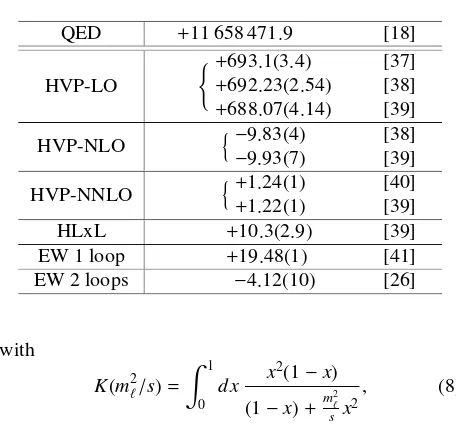
The contribution known as hadronic vacuum polarization (HVP) occurs first at orderO(α2), cf. Fig. 1. This lowest-order HVP contribution (aHVPµ −LO) provides the largest hadronic correction to aµ, but also, to date, one of the largest contribution to the theoretical uncertainty (see Ta-ble 1). aHVPµ −LO can be expressed in the following way [29–31]
aHVPℓ −LO=1 3
α
π
2 ∞
4M2
π
ds s
m2ℓ
s K(m 2 ℓ/s)R
had
Table 1.The contributions toaµ(in units of 10−10) using the latest available values
QED +11 658 471.9 [18]
HVP-LO
+693.1(3.4) +692.23(2.54) +688.07(4.14)
[37] [38] [39]
HVP-NLO −9.83(4)
−9.93(7)
[38] [39]
HVP-NNLO +1.24(1) +1.22(1)
[40] [39]
HLxL +10.3(2.9) [39]
EW 1 loop +19.48(1) [41]
EW 2 loops −4.12(10) [26]
with
K(m2ℓ/s)= 1
0
dx x 2(1−x)
(1−x)+m 2
ℓ s x2
, (8)
andRhad(s) represents theR-ratio of the cross section for e+e−→
hadrons. This contribution can therefore be evalu-ated using available experimental input. Actually, as illus-trated by the second diagram (b) in Fig. 1, what is usually refered to as HVP-LO contains some contributions at order
O(α3), for instance the radiative modese+e− → π0γ, ηγ . The remainingO(α) [O(α2)] QED corrections to Fig. 1 are descibed as next-to-leading HVP (HVP-NLO) [next-next-to-leading HVP (HVP-NNLO)].
Previous data-based evaluations of aLO−HVP
µ had
reached a precision around 0.6% [32–34]. Recently, three new evaluations have been made. Their results, shown in Table 1, are in agreement within the uncertainties given. They include new data (for the experimental aspects, see
(a) (b)
Figure 1. Diagrammatic representation ofaHVP−LO
µ , the leading hadronic vacuum polarization contribution toaµ. In diagram (a), the shaded blob represents the�VV�QCD two-point function. Also shown is a next-to-leading contribution, diagram (b), actu-ally included inaHVP−LO
µ (see text).
Table 2.The contribution toaHVP−LO
µ (in units of 10−10) coming from the measurement of thee+e−→
π+π−cross section in the region between 600 and 900 MeV. Values taken from Fig. 7 in
Ref. [42]. Experiment aHVP−LO 2π
µ (600−900 MeV) BaBar(09) 376.7(2.7)
KLOE(comb) 366.9(2.1) BESIII(15) 368.2(4.2) SND(04) 371.7(5.0) CMD-2(comb) 372.4(3.0)
Table 3.Some recent lattice evaluations ofaHVP−LO
µ (in units of 10−10). The first error is the statistical one, the second the
systematic one. 654±32+21
−23 [43]
667±6±12 [44] 711.0±7.5±17.3 [45] 715.4±16.3±9.2 [46]
[35, 36]), and reach now a precision around 0.4%. How-ever, some tension remains between the high-precision e+e− → π+π− data collected in the region of the ρ
res-onance, for instance, by BaBar on the one side, and by KLOE and BESIII on the other side, as shown in Table 2 (see also [35]). From a general point of view, given the very high precision achieved, and even more so in view of this tension in the data, some cross-checks would be welcome here also. Several proposal in this direction have been put forward, and are worth investigating.
For one thing, it has been proposed to evaluate the vacuum polarization integral using data not from the time-like region, but from the space-time-like one, i.e. by consider-ing either Bhabha scatterconsider-ing [48], or muon-electron scat-tering [49]. While the required statistical accuracy could be reached upon operating for two years at, for instance, the muon beam of 150 GeV available at the CERN North Area, getting the systematic uncertainties below the re-quired level of about 10 ppm constitutes a real challenge. The issue of controling higher-order radiative corrections will also be crucial. The latter aspect has been discussed in several presentations [50–53] at this Worshop, to which I refer the interested reader.
Staying in the Euclidian region, there has been grow-ing interest in the lattice-QCD community to compute aHVPµ −LO through numerical simulations. Several results have appeared since the first FCCP meeting in 2015, and are summarized in Table 3. The precision is still too low, around 2.5% or more, in order to be competitive with the determinations based on the e+e− → hadrons
data. Moreover, the systematic uncertainties indicated cover different realities as far as the control over lattice artefacts and/or isospin-breaking effects (see e.g. [47]) is concerned. Nevertheless, the situation looks promis-ing, and one might also consider, as done by the au-thors of Ref. [46], replacing experimental data by lat-tice data in the energy regions where the latter are more accurate. Supplementing lattice data for very short and very long distances with experimental measurements of Rhad(s), the value shown in the last entry of Table 3 be-comesaHVPµ −LO=692.5(1.4)(0.5)(0.7)(2.1)·10−10, where the two first errors come from the lattice, the two last ones from experiment. Combining all these uncertainties in quadrature leads to an overall relative error of less than 0.4%!
K(κ) in (8). From the simple inequalities
f(x;κ0)< f(x;κ)< κx2[1−κx2(1−x)], (9)
valid within the ranges of variation of bothxandκ, one ob-tains the bounds (keeping only the first term on the right-hand side of the second inequality reproduces the upper bound obtained long ago in Ref. [57])
α
πK(κ0)M(0)<a
HVP−LO
ℓ <
α π
1
3[M(0)− 11
10M(−1)], (10) in terms of the moments of the Mellin-Barnes transform of the imaginary part of the vacuum polarization function [54],
M(y)= � ∞
4M2
π
ds s
m2ℓ
s
y−1 1
πImΠ(s),
1
πImΠ =
1 3
α πR
had
.
(11) Using, for illustrative purposes, the simple toy model for Rhad(s) given in Ref. [58], one finds, in the case of the elec-tron, very stringent lower and upper bounds, which in both cases deviate from the actual value given by the toy model by less than 0.1%. The situation in less favourable in the case of the muon. The lower bound amounts to about only 70% of the actual value, and the upper bound exceeds it by 12%. In order to move beyond the simple bounds of the type shown above requires to use more elaborate mathe-matical techniques. This has been done by the authors of Refs. [54–56], who obtain a rapidly converging represen-tation in terms of a series of the type
aHVPµ −LO=�
n≥0
[cnM(−n)+c′nM ′
(−n)], (12)
involving not only M(s), but also its derivative M′(s).
Only a few terms of this series can already provide an evaluation that differs from the full result by less that 1%. The corresponding moments can be determined from phe-nomenology [59], or computed on the lattice [60].
5 Progress in the evaluation of the
hadronic light-by-light (HLxL)
Hadronic light-by-light scattering is the next important hadronic contribution to aµ. It involves the fourth-rank vacuum polarization tensor, as shown on Fig. 2. In con-trast to the two-point hadronic vacuum polarization tensor involved inaHVPµ −LO, there is, in the case ofaHLxLµ , no sim-ple and direct link to an experimental observable, similar to Eq. (7). Other strategies must then be devised in order to overcome the difficulties in handling strong-interaction effects in the non-perturbative regime, while keeping the amount of model dependence at the lowest possible level. Two approaches that can potentially fulfill this condition have been developped in order to evaluateaHLxL
µ : disper-sion relations and numerical simulations of QCD on the lattice.
The dispersive framework set up in Refs. [61, 62] uses a decomposition of the fourth-rank vacuum polarization
Figure 2. The hadronic light-by-light contribution toaµ. The blob represents the hadronic fourth-rank polarization tensor, i.e. vaccun expectation value of the time-ordered product of four hadronic electromagnetic currents.
tensor into independent invariant functions free of kine-matic zeroes and of singularities, for which dispersion re-lations can be written. These dispersion rere-lations can then be saturated by one-, two- or more meson states and ex-pressed in terms of corresponding form factors. The latter can furthermore be obtained from experiment [63, 64] or again... from lattice QCD [65, 66]. Applying this for-malism to theππintermediate state [67] [68] provides not only a new evaluation of the so-called pion box contribu-tion (see also Ref. [69] for a recent discussion of this con-tribution), but includes also S-wave rescattering effects. The result obtained this way is very accurate, at the 4% level. Results concerning other contributions are to be ex-pected in the future. What is so far missing in this disper-sive approach, is how QCD short-distance properties [70] (see also the discussion of this issue in [11]) of the fourth-rank vacuum polarization tensor will eventually be imple-mented in this formalism, that is how the various individ-ual contributions will be put together in order to reproduce the correct high-energy behaviour.
Two groups are at present actively involved in the com-putation ofaHLxL
µ from lattice QCD [71–75]. The authors of Ref. [72] obtainaHLxL
µ =5.35(1.35)·10
−10, where the
error is statistical only (finite-volume effects are discussed in Ref. [73]). Although the central value lies somewhat on the low side as compared to current phenomenological es-timates [34, 76], this new result opens promising prospects for the future.
6 Conclusion
The Fermilab g-2 experiment will very soon measure the anomalous magnetic moment of the muon with a precision comparable to the Brookhaven experiment, and, within a couple of years will reduce its uncertainty by a factor or four. Hopefully, the J-PARC experiment E34, which is based on a completely different set-up, will later on pro-vide a cross-check of this important measurement.
QED provides, by far, the largest contribution toaµ, and even more so to ae. All numerical evaluations of
the contributions at fourth order have now been satisfacto-rily cross-checked by analytical tools, including the mass-independent one, so crucial for ae. The only potential
The data-based determinations of the contribution to aµfrom hadronic vacuum polarization have been improved thanks to new high-precision experimental input, and more data should become available in the near future, hope-fully helping in removing some tensions between diff er-ent experimer-ents. Cross-checks coming from different ap-proaches seem to be possible. Extracting the vacuum po-larization function fromµescattering constitutes an inter-esting proposal in this direction, although the control of the systematic effects represents a quite challenging issue. Interesting developments have also come from numerical simulations of QCD on the lattice. Improvements in the statistical precision and increased control over systematic effects are still needed in order to compete with the data-based determinations. Of particular interest is the possi-bility to combine data and lattice results, taking advantage of the performance of each in various energy regions.
Progress in the determination of the HLxL contribu-tion has been made both in the dispersive approach, and in lattice QCD. The dispersive approach offers the possibility to make use of experimental data or lattice results for var-ious form factors. The results obtained so far are encour-aging, and confirm that no important physical effect has been overlooked by the existing phenomenological evalu-ations. The issue here will rather consist in improving on the present precision and in obtaining reliable estimate of the uncertainties due to lattice artefacts.
Acknowledgements
I would like to thank the organizers of the Work-shop “Flavour changing and conserving processes 2017” for the kind invitation to participate to this second FCCP Workshop, and for choosing the perfect place for such a meeting. This work has been partially supported by the OCEVU Labex (ANR-11-LABX-0060) and the A*MIDEX project (ANR-11-IDEX-0001-02) funded by the "Investissements d’Avenir" French government pro-gram managed by the ANR.
References
[1] D. Hanneke et al., Phys. Rev. Lett. 100, 120801 (2008).
[2] G. W. Bennett et al., Phys. Rev D73, 072003 (2006). [3] C. Patrignani et al. [Particle Data Group], Chin. Phys.
C40, 100001 (2016).
[4] G.A. González-Sprinberg et al., Nucl. Phys. B582, 3 (2000).
[5] S. Narison, Phys. Lett. B513, 53 (2001); Err. B526, 414 (2002)
[6] J. Abdallah et al. [DELPHI Coll.], Eur. Phys. J. C35, 158 (2004).
[7] S. Eidelman, M. Passera, Mod. Phys. Lett. A22, 159 (2007).
[8] J. Bernabéu et al., Nucl. Phys. B790, 160 (2008). [9] S. Eidelman et al., (2016).
[10] G. D’Ambrosio, M. Iacovacci, M. Passera, G. Venan-zoni, P. Massarotti and S. Mastroianni, EPJ Web Conf.
118(2016).
[11] M. Knecht, EPJ Web Conf.118, 01017 (2016). [12] R. M. Carey et al.. The New g-2 experiment - 2009.
Fermilab. Proposal 0989.
[13] B. Lee Roberts, Chin. Phys. C34, 741 (2010). [14] See the contribution of T. Gorringe to this workshop. [15] T. Mibe [J-PARC g-2 Collaboration], Chin. Phys. C
34, 745 (2010).
[16] See the contribution of G. Marshall to this workshop. [17] See the contribution of S. Laporta to this workshop. [18] T. Aoyama et al, Phys. Rev. Lett.109, 111808 (2012)
[arXiv:1205.5370 [hep-ph]].
[19] T. Aoyama et al, Prog. Theor. Exp. Phys. 2012, 01A107 (2012).
[20] T. Aoyama et al, Phys. Rev. D 91, 033006 (2015); Phys. Rev. D96, 019901(E) (2017).
[21] A. Kurz et al., Phys. Rev. D92, no. 7, 073019 (2015) [arXiv:1508.00901 [hep-ph]].
[22] A. Kurz et al., Phys. Rev. D93, no. 5, 053017 (2016) [arXiv:1602.02785 [hep-ph]].
[23] M. Beneke and V. A. Smirnov, Nucl. Phys. B 522, 321 (1998) [hep-ph/9711391].
[24] V. A. Smirnov, Springer Tracts Mod. Phys. 177, 1 (2002).
[25] A. Kurz et al., Nucl. Phys. B 879, 1 (2014) [arXiv:1311.2471 [hep-ph]].
[26] C. Gnendiger et al., Phys. Rev. D88, 053005 (2013) [arXiv:1306.5546 [hep-ph]].
[27] R. Bouchendira et al., Phys. Rev. Lett.106, 080801 (2011).
[28] S. Laporta, Phys. Lett. B772, 232 (2017).
[29] C. Bouchiat and L. Michel, J. Phys. Radium 22, 121 (1961).
[30] L. Durand, Phys. Rev. 128, 441 (1962); Err.-ibid.
129, 2835 (1963).
[31] M. Gourdin and E. de Rafael, Nucl. Phys. B10, 667 (1969).
[32] M. Davier et al., Eur. Phys. J. C71, 1515 (2011) [Eur. Phys. J. C 72, 1874 (2012)] [arXiv:1010.4180 [hep-ph]].
[33] K. Hagiwara et al., J. Phys. G 38, 085003 (2011) [arXiv:1105.3149 [hep-ph]].
[34] F. Jegerlehner and R. Szafron, Eur. Phys. J. C 71, 1632 (2011) [arXiv:1101.2872 [hep-ph]].
[35] See the contribution of F. Ignatov to this workshop. [36] See the contribution of A. Denig to this workshop. [37] M. Davier et al., Eur. Phys. J. C 77, 827 (2017)
[arXiv:1706.09436 [hep-ph]].
[38] See the contribution of D. Nomura to this workshop. [39] F. Jegerlehner, EPJ Web Conf. 166, 00022 (2018)
[arXiv:1705.00263 [hep-ph]].
[40] A. Kurz et al., Phys. Lett. B 734, 144 (2014) [arXiv:1403.6400 [hep-ph]].
[42] A. Anastasi et al. [KLOE-2 Collaboration], arXiv:1711.03085 [hep-ex].
[43] M. Della Morte et al., JHEP 1710, 020 (2017) [arXiv:1705.01775 [hep-lat]].
[44] B. Chakraborty et al. [HPQCD coll.], Phys. Rev. D
96, no. 3, 034516 (2017) [arXiv:1601.03071 [hep-lat]]. [45] S. Borsanyi et al. [Budapest-Marseille-Wuppertal
coll.], arXiv:1711.04980 [hep-lat].
[46] T. Blumet al., arXiv:1801.07224 [hep-lat]. [47] P. Boyle et al., arXiv:1710.07190 [hep-lat].
[48] C. M. Carloni Calame et al., Phys. Lett. B746, 325 (2015) [arXiv:1504.02228 [hep-ph]].
[49] G. Abbiendi et al., Eur. Phys. J. C 77, 139 (2017) [arXiv:1609.08987 [hep-ex]].
[50] See the contribution of L. Trentadue to this work-shop.
[51] See the contribution of U. Marconi to this workshop. [52] See the contribution of P. Mastrolia to this workshop. [53] See the contribution of F. Piccinini to this workshop. [54] E. de Rafael, Phys. Lett. B 736, 522 (2014)
[arXiv:1406.4671 [hep-lat]].
[55] E. de Rafael, Phys. Rev. D96, no. 1, 014510 (2017) [arXiv:1702.06783 [hep-ph]].
[56] J. Charles et al., arXiv:1712.02202 [hep-ph]. [57] J. S. Bell and E. de Rafael, Nucl. Phys. B 11, 611
(1969).
[58] D. Bernecker and H. B. Meyer, Eur. Phys. J. A47, 148 (2011) [arXiv:1107.4388 [hep-lat]].
[59] M. Benayoun et al, arXiv:1605.04474 [hep-ph]. [60] S. Borsanyiet al., Phys. Rev. D96, 074507 (2017)
[arXiv:1612.02364 [hep-lat]].
[61] G. Colangelo et al.,JHEP 1409, 091 (2014) [arXiv:1402.7081 [hep-ph]].
[62] G. Colangelo et al., JHEP 1509, 074 (2015) [arXiv:1506.01386 [hep-ph]].
[63] G. Colangelo et al., Phys. Lett. B 738, 6 (2014) [arXiv:1408.2517 [hep-ph]].
[64] A. Nyffeler, Phys. Rev. D94, no. 5, 053006 (2016) doi:10.1103/PhysRevD.94.053006 [arXiv:1602.03398 [hep-ph]].
[65] X. Feng et al., Phys. Rev. D91, no. 5, 054504 (2015) [arXiv:1412.6319 [hep-lat]].
[66] A. Gérardin et al., Phys. Rev. D 94, no. 7, 074507 (2016) [arXiv:1607.08174 [hep-lat]].
[67] G. Colangelo et al., Phys. Rev. Lett. 118, no. 23, 232001 (2017) [arXiv:1701.06554 [hep-ph]].
[68] G. Colangelo et al., JHEP 1704, 161 (2017) [arXiv:1702.07347 [hep-ph]].
[69] J. Bijnens and J. Relefors, JHEP 1609, 113 (2016) [arXiv:1608.01454 [hep-ph]].
[70] K. Melnikov and A. Vainshtein, Phys. Rev. D 70, 113006 (2004).
[71] J. Green et al., PoS LATTICE 2015, 109 (2016) [arXiv:1510.08384 [hep-lat]].
[72] T. Blum et al, Phys. Rev. Lett. 118, 022005 (2017) [arXiv:1610.04603 [hep-lat]].
[73] T. Blum et al., Phys. Rev. D 96, 034515 (2017) [arXiv:1705.01067 [hep-lat]].