Computational Information Geometry For Binary Classification of High-Dimensional Random Tensors

Computational Information Geometry For Binary

Classification of High-Dimensional

Random Tensors

†

Gia-Thuy Pham1, Rémy Boyer1and Frank Nielsen2,3,*

1 _{University of Paris-Sud, L2S, Department of Signals and Statistics, France;}

[email protected] (G.-T.P.); [email protected] (R.B.) 2 _{École Polytechnique, LIX, France}

3 _{Sony Computer Science Laboratories, Japan}

* Correspondence: [email protected]; Tel.: +x-xxx-xxx-xxxx

† The results presented in this work have been partially published in [16] and [15]

Abstract: The performance in terms of minimal Bayes’ error probability for detection of a high-dimensional random tensor is a fundamental under-studied difficult problem. In this work, we consider two Signal to Noise Ratio (SNR)-based detection problems of interest. Under the alternative hypothesis,i.e., for a non-zero SNR, the observed signals are either a noisy rank-Rtensor admitting a

Q-order Canonical Polyadic Decomposition (CPD) with large factors of sizeNq×R,i.e, for 1≤q≤Q,

whereR,Nq → ∞withR1/q/Nq converge towards a finite constant or a noisy tensor admitting

TucKer Decomposition (TKD) of multilinear(M1, . . . ,MQ)-rank with large factors of sizeNq×Mq, i.e,for 1≤q≤Q, whereNq,Mq →∞withMq/Nqconverge towards afiniteconstant. The detection

of the random entries (coefficients) of the core tensor in the CPD/TKD is hard to study since the exact derivation of the error probability is mathematically intractable. To circumvent this technical difficulty, the Chernoff Upper Bound (CUB) for larger SNR and the Fisher information at low SNR are derived and studied, based on information geometry theory. The tightest CUB is reached for the value minimizing the error exponent, denoted bys?. In general, due to the asymmetry of the

s-divergence, the Bhattacharyya Upper Bound (BUB) (that is, the Chernoff Information calculated at

s?=1/2) can not solve this problem effectively. As a consequence, we rely on a costly numerical optimization strategy to finds?. However, thanks to powerful random matrix theory tools, a simple analytical expression ofs?is provided with respect to the Signal to Noise Ratio (SNR) in the two schemes considered. A main conclusion of this work is that the BUB is the tightest bound at low SNRs. This property is, however, no longer true for higher SNRs.

Keywords: Optimal Bayesian detection, information geometry, minimal error probability, Chernoff/Bhattacharyya upper bound, large random tensor, Fisher information, large random sensing matrix

1. Introduction

1.1. State-of-the-art and problem statement

Evaluating the performance limit for the “Gaussian information plus noise” detection problem is a challenging research topic, see for instance [6,8,9,34,36,39,46]. Given a binary hypothesis problem, the Bayes’ decision rule is based on the principle of the largest posterior probability. Specifically, the Bayesian detector chooses the alternative hypothesisH₁ if Pr(H₁|y) > Pr(H₀|y) for a given

N-dimensional measurement vectoryor the null hypothesisH0, otherwise. Consequently, the optimal

decision rule can often only be derived at the price of a costly numerical computation of the log posterior-odds ratio [34] since an exact calculation of the minimal Bayes’ error probability Pe(N)is

often intractable [17,34]. To circumvent this problem, it is standard to exploit well-known bounds on Pe(N)based on information theory [2,24,32,42,47]. In particular, theChernoff information[19,40]

is asymptotically (inN) relied to the exponential rate ofPe(N). The Chernoff information turns out

to be useful in many problems of practical importance as for instance, distributed sparse detection [18], sparse support recovery [48], energy detection [35], MIMO radar processing [31,45], network secrecy [13], Angular Resolution Limit in array processing [27], detection performance for informed communication systems [33], just to name a few. In addition, the Chernoff information bound can be tight for a minimal s-divergence over parameter s ∈ (0, 1). Generally, this step requires to solve numerically an optimization problem [41] and often leads to a complicated and uninformative expression of the optimal value ofs. To circumvent this difficulty, a simplified case ofs=1/2 is often used corresponding to the well-known Bhattacharyya divergence [47] at the price of a less accurate prediction ofPe(N). In information geometry, parametersis often calledα, and thes-divergence is the so-called Chernoffα-divergence [41].

The theory of tensor decomposition is a timely and important research topic [20,23]. Tensors are useful to extract relevant information confined into a small dimensional subspace from a massive and multidimentional volume of measurements. In the standard literature, two main families of tensor decomposition are prominent. Namely the Canonical Polyadic Decomposition (CPD) [23] and the Tucker decomposition (TKD)/HOSVD (High-Order SVD) [25,49]. These approaches are two possible multilinear generalization of the Singular Value Decomposition (SVD). A natural generalization to tensors of the usual concept of rank for matrices is called the CPD. The tensorial/canonical rank of a

P-order tensor is equal to the minimal positive integer, sayR, of unit rank tensors that must be summed up for perfect recovery. A unit rank tensor is the outer product ofPvectors. In addition, the CPD has remarkable uniqueness properties [23] and involves only a reduced number of free parameters due to the constraint of minimality onR. Unfortunately, unlike to the matrix case, the set of tensors with fixed (tensorial) rank is not close [21,26]. This singularity implies that the problem of the computation of the CPD is mathematically ill-posed. The consequence is that its numerical computation remains non trivial and is usually done using suboptimal iterative algorithms [22]. Note that this problem can sometimes be avoided by exploiting some natural hidden structures in the physical model [30]. The TKD [49] and the HOSVD [25] are two popular decompositions being an alternative to the CPD. In this case, the notion of tensorial rank is no longer relevant and a new rank definition is used. Specifically, it is standard to use themultilinear rankdefined as the set of positive integers{R1, . . . ,RP}where each

integer,Rp, is the usual rank of thep-th mode. Its practical construction is non-iterative and optimal in

the sense of the Eckart-Young theorem at each mode level. This approach is interesting because it can be computed in real-time [4] or adaptively [12]. Unfortunately, it is shown that the low (multilinear) rank tensor based on this procedure is generally suboptimal [25]. In other words, there does not exist a generalization of the Eckart-Young theorem for tensors of order strictly greater than two!

The detection performance of a multilinear tensor following the CPD and TKD can be derived and studied. It is important to note that the detection theory for tensors is a very under studied research topic. To the best of our knowledge, only the publication [10] tackles this problem in the context of RADAR multidimensional data detection. A major difference with this publication is that their analysis is based on the performance of a low rank detection after matched filtering.

More specifically, we consider two cases where the observations are either (1) a noisy rank-Rtensor admitting a Q-order CPD with large factors of size Nq×R, i.e, for 1 ≤ q ≤ Q, R,Nq → ∞with R1/q_/N

qconverging towards a finite constant, or (2) a noisy tensor admitting a TKD of multilinear (M1, . . . ,MQ)-rank with large factors of sizeNq×Mq,i.e., for 1 ≤q≤ Q, whereNq,Mq →∞with Mq/Nqconverging towards a finite constant. For zero-mean independent Gaussian core and noise

tensors a key discriminative parameter is the Signal to Noise Ratio defined by SNR=σ_s2/σ2whereσ_s2 andσ2are the variances of the vectorized core and noise tensors, respectively. So, the binary hypothesis test of interest can be described in the following way:

Under the null hypothesisH0, SNR = 0, meaning that only the noise is present. Conversely,

for tensors. The detection of the random entries of the core tensor is hard to study since the exact derivation of the error probability is intractable. To circumvent this technical difficulty, based on computational information geometry theory, we consider the Chernoff Upper Bound (CUB), and the Fisher information in the context of massive measurement vectors. The tightest CUB is reached for the value, denoted bys?, which minimizes the error exponent. In general, due to the asymmetry of thes-divergence, the Bhattacharyya Upper Bound (BUB) — Chernoff Information calculated at

s? =1/2— cannot solve this problem effectively. As a consequence, we rely on a costly numerical optimization strategy to finds?. However, thanks to powerful Random Matrix Theory (RMT) tools, a simple analytical expression ofs?is provided with respect to the Signal to Noise Ratio (SNR). For low SNR, analytical expressions of the Fisher information are given. Note that the analysis of the Fisher information in the context of the RMT has been only studied in recent contributions [11,14,43] for parameter estimation. For larger SNR, analytic and simple expression of the CUB for the CPD and the TKD are provided.

We note that Random Matrix Theory (RMT) has fascinated both mathematicians and physicists since they were first introduced in mathematical statistics by Wishart in 1928 [54]. After a slow start, the subject gained prominence when Wigner [52] introduced the concept of statistical distribution of nuclear energy levels in 1950. However, it took until 1955 before Wigner [53] introduced ensembles of random matrices. Since then, many important results in RMT were developed and analyzed, see for instance [5,29,38,51] and the references therein. In the last two decades, researches on RMT has been constantly published.

1.2. Paper organisation

The organization of the paper is as follows: In the second section, we introduce some definitions, tensor models, and the Marchenko-Pastur distribution from random matrix theory. The third section is devoted to present Chernoff Information for binary hypothesis test. The fourth section gives the main results on Fisher Information and the Chernoff bound. The numerical simulation results are given in the fifth section. We conclude our work by giving some perspectives in the Section 6. Finally, several proofs of the paper can be found in the appendix. We also give the list of theorem, result, lemma, remark and definitions.

List of Theorems

1 Definition . . . 4

2 Definition . . . 4

3 Definition . . . 4

4 Definition . . . 4

6 Lemma . . . 9

7 Lemma . . . 9

8 Lemma . . . 9

9 Result. . . 10

10 Remark . . . 11

11 Result. . . 11

12 Result. . . 11

13 Remark . . . 11

14 Result. . . 12

15 Result. . . 13

16 Remark . . . 13

17 Result. . . 13

18 Result. . . 14

2. Algebra of tensors and Random Matrix Theory (RMT)

In this section, we introduce some useful definitions from tensor algebra and from the spectral theory of large random matrices.

2.1. Multilinear functions

2.1.1. Preliminary definitions

Definition 1. The Kronecker product of matricesXandYof size I×J and K×N, respectively is given by

X⊗Y= 

 

[X]11Y . . . [X]1JY ..

. ...

[X]I1Y . . . [X]I JY 

 ∈R

(IK)×(JN)_.

We have rank{X⊗Y}=rank{X} ·rank{Y}.

Definition 2. The vectorizationvec(X)of a tensorX ∈RM1×...×MQ is a vectorx∈RM1M2...MQ defined as xh= [X]m₁,...,m_Q

where h=m1+_∑Q_k=2(mk−1)M1M2...Mk−1.

Definition 3.The q-mode product denoted by×qbetween a tensorX ∈RM1×...×MQand a matrixU∈RK×Mq is denoted byX×qU∈RM1×...×Mq−1×K×Mq+1×...×MQwith

[X ×qU]m1,...,mq−1,k,mq+1,...,mQ =

Mq

∑

[X]m1,...,mQ[U]k,mq

where1≤k≤K.

Definition 4. The q-mode unfolding matrix of size Mq×

∏Q

k=1,k6=qMk

denoted byX(q)=unfoldq(X)of a tensorX ∈RM1×...×Mq is defined according to

[X(q)]Mq,h= [X]m1,...,mQ

where h=1+_∑kQ_=1,k6=q(mk−1)∏k_v−₌1_1,v6=qMv.

2.1.2. Canonical Polyadic Decomposition (CPD)

The rank-RCPD of orderQis defined according to

X =

R

∑

sr

φr(1)◦. . .◦φ(rQ)

| {z }

Xr

with rank{Xr}=1

where◦is the outer product [20],φ(rq)∈RNq×1andsris a real scalar.

An equivalent formulation using theq-mode product defined in Def.3is

X =S×₁Φ(1)_×

2. . .×QΦ(Q)

whereSis theR× · · · ×Rdiagonal core tensor with[S]r,...,r =sr andΦ(q)= [φ(₁q)...φ(_Rq)]is theq-th factor matrix of sizeNq×R.

X(q)=Φ(q)S

Φ(Q)_...Φ(q+1)_Φ(q−1)_...Φ(1)T

whereS=diag(s)withs= [s1, ...,sR]Tandstands for the Khatri-Rao product [20].

2.1.3. Tucker Decomposition (TKD)

The Tucker tensor model of orderQis defined according to

X =

M1

∑

M2

∑

...

MQ

∑

sm1m2...mQ

φ(m11)◦φ

(2)

m2 ◦ · · · ◦φ

(Q)

mQ

whereφ(mqq)∈R

Nq×1_{,q=1, ...,Qands}

m1m2...mQis a real scalar.

Theq-mode product ofX is similar to CPD case, however theq-mode unfolding matrix for tensorX

is slightly different

X(q)=Φ(q)S(q)

Φ(Q)_{⊗. . .⊗Φ}(q+1)_⊗Φ(q−1)_{. . .⊗Φ}(1)T

whereS(q)∈RNq×N1N2...Nq−1Nq+1...NQtheq-mode unfolding matrix of tensorS,Φ(q)= [φ₁(q)...φ(_Mq)_q]∈

RNq×Mq and⊗stands for Kronecker product.

Figure 1.Canonical Polyadic Decomposition (CPD)

At this point, it is important to note that the CPD and TKD formalism implies that vectorxin (11) is related either to the structured linear systemΦorΦ⊗.

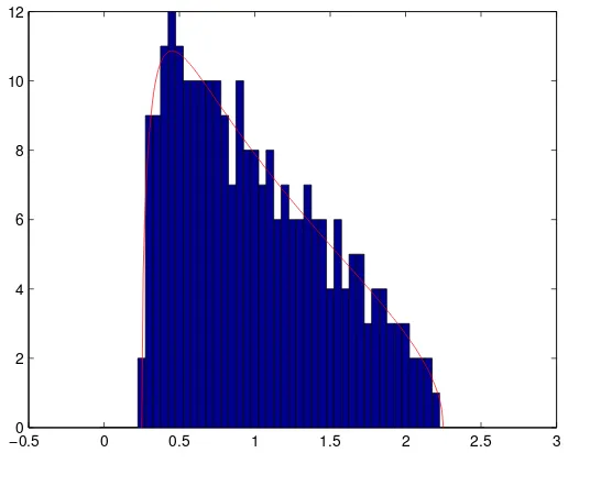
2.2. The Marchenko-Pastur distribution

The Marchenko-Pastur distribution was introduced half a century ago [38] in 1967, and plays a key role in a number of high-dimensional signal processing problems. To help the reader, in this section, we introduce some fundamental results concerning large empirical covariance matrices. Let(vn)n=1,...,Na

sequence of i.i.d zero mean Gaussian random M-dimensional vectors for whichE(vnvTn) =σ2IM. We

consider the empirical covariance matrix

1

N N

∑

vnvnT

which can be also written as

1

N N

∑

where matrixWNis defined byWN = √1_N[v1, ...,vN].WNis thus a Gaussian matrix with independent

identically distributedN(0,σ2

N) entries. When N → +∞while Mremains fixed, matrixWNWTN

converges towardsσ2IMin the spectral norm sense. In the high dimensional asymptotic regime

defined by

M→+∞, N→+∞, cN= M

N →c>0

it is well understood that WNW

T

N−σ2IM

does not converge towards 0. In particular, the empirical distribution ˆνN = _M1 ∑Mm=1δ_λˆ_m,N of the eigenvalues ˆλ1,N ≥... ≥λˆM,NofWNWTNdoes not converge

towards the Dirac measure at pointλ=σ2. More precisely, we denote byν_c,σ2 the Marchenko-Pastur

distribution of parameters(c,σ2)defined as the probability measure

ν_c,σ2(dλ) =δ0[1−1 c]++

p

(λ−λ−)(λ+−λ) 2σ2cπλ 1[λ

−_,λ+_](λ)dλ (1)

withλ−=σ2(1− √

c)2andλ+ =σ2(1+ √

c)2. Then, the following result holds.

Theorem 5. ([38]) The empirical eigenvalue value distributionµˆNconverges weakly almost surely towards µ_d,σ2 when both M and N converge towards +∞in such a way that cN = MN converges towards c > 0. Moreover, it holds that

ˆ

λ1,N →σ2(1+√c)2a.s. (2)

ˆ

λ_min(M,N) →σ2(1− √

c)2a.s. (3)

−0.5 0 0.5 1 1.5 2 2.5 3 0

10 20 30 40 50 60 70

Figure 2.Histogram of the eigenvalues ofWNWTN

−0.5 0 0.5 1 1.5 2 2.5 3 0

2 4 6 8 10 12

Figure 3.Histogram of the eigenvalues ofWNWTN

N (withM=256,cN= MN = 14,σ2=1)

We also observe that Theorem5remains valid ifWNis not necessarily a Gaussian matrix whose

i.i.d. elements have a finite fourth order moment (see e.g. [5]). Theorem5means that when ratio M_N is not small enough, the eigenvalues of the empirical spatial covariance matrix of a temporally and spatially white noise tend to spread out around the variance of the noise, and that almost surely, forN

large enough, all the eigenvalues are located in a neighbourhood of interval[λ−,λ+].

3. Classification in a Computational Information Geometry (CIG) framework

3.1. Formulation based on aSNR-type criterion

Let SNR=σ_s2/σ2andpi(·) =p(·|Hi)withi∈ {0, 1}. The equi-probable binary hypothesis test

for the detection of the random signal,s, is (

H0:p0(yN;Φ, SNR=0) =N(0,Σ0), H1:p1(yN;Φ, SNR6=0) =N(0,Σ1)

(4)

whereΣ0 = σ2IN andΣ1 = σ2

SNR·ΦΦT+IN

. The data-space for the null hypothesis (H0) is

given byX0=X \ X1where

X1=

yN:Λ(yN) =logp1(yN ) p0(yN)

>τ0

is the data-space for the alternative hypothesis (H₁). In the above test,Λ(yN)is the log likelihood ratio

test andτ0is the detection threshold given by the following two expressions:

Λ(yN) =

yT_NΦΦTΦ+SNR·I−1ΦTyN

σ2 ,

τ0=−log det

SNR·ΦΦT_+I N

3.2. Geometry of the expected log-likelihood ratio

Consider p(yN

H) =ˆ N(0,Σ) associated to the estimated hypothesis ˆH. The expected log-likelihood ratio is given by

E_y

N

HˆΛ(yN) =

Z

X p(yN

H)ˆ log

p1(yN) p0(yN)dyN =KL(H||Hˆ 0)− KL(H||Hˆ 1)

= 1 σ2Tr

ΦT_Φ+SNR·I−1_ΦT_ΣΦ

where

KL(H||Hˆ _i) =

Z

X p(yN

H)ˆ log

p(yN H)ˆ pi(yN)

dyN

is the Kullback-Liebler Divergence (KLD) [24]. The expected log-likelihood ratio test admits to a simple geometric characterization based on the difference of two KLDs [17]. But, the performance of the detector of interest in terms of the minimal Bayes’ error probability, denoted byPe(N), is quite often

difficult to determine analytically [17,34] in closed-form.

Define the minimal Bayes’ error probability conditionally to vectoryNaccording to

Pr(Error|yN) =

1

2min{P1,0,P0,1} wherePi,i0 =Pr(H_i|y_N∈ X_i0).

3.3. CUB

The (average) minimal Bayes’ error probability defined by Pe(N) = EPr(Error|yN) is upper

bounded according to the CUB [41] such as

Pe(N)≤ 1

2·exp[−µN(s)] (5)

where the (Chernoff)s-divergence fors∈(0, 1)is given by

µN(s) =−logMΛ(yN|H1)(−s) (6)

in whichMX(t) =Eexp[t·X]is themoment generating function(mgf) of variableX. The error exponent,

denoted byµ(s), is given by the Chernoff information which is an asymptotic characterization on the exponentially decay of the minimal Bayes’ error probability. The error exponent is derived thanks to the Stein’s lemma according to [47]

− lim

N→∞

logPe(N)

N =Nlim→∞

µN(s) N

def. = µ(s).

As parameters∈(0, 1)is free, the CUB can be tightened by minimizing this parameter:

s?=arg min

Finally using eq. (5) and eq. (7), we obtain the Chernoff Upper Bound (CUB). The Bhattacharyya Upper Bound (BUB) is obtained by eq. (5) and by fixings=1/2 instead of solving eq. (7). Therefore we have the following relation of order:

Pe(N)≤ 1

2·exp[−µN(s

?_)]≤ 1

2·exp[−µN(1/2)].

Lemma 6. The log-moment generating function given by eq.(6)for test of eq.(4)is given by

µN(s) =

1−s

2 log det

SNR·ΦΦT_{+I (8)}

−1

2log det

SNR·(1−s)ΦΦT+I.

Proof. See Appendix7.1

3.4. Fisher information

In the small deviation regime, we assume thatδSNR is a small deviation of the SNR. The new binary hypothesis test is

(

H0 : y|δSNR=0∼ N(0,Σ(0)), H1 : y|δSNR6=0∼ N

0,Σ(δSNR)

whereΣ(x) =x·ΦΦT_{+I. Thes-divergence in the small SNR deviation scenario is written as}

µN(s) =1 −s

2 log det[Σ(δSNR)]− 1

2log det[Σ(δSNR·(1−s))]

Lemma 7. The s-divergence in the small deviation regime can be approximated according to µN(s)

N

δSNR1

≈ (s−1)s·(δSNR) 2

2 ·

JF(0) N where the Fisher information [34] is given by

JF(x) = 1

2Tr((I+x·ΦΦ

T₎−1_ΦΦT_(I+x·ΦΦT₎−1_ΦΦT_).

Proof. See Appendix7.2

According to Lemma7, the optimals-value at low SNR iss?δSNR=1 1₂. At contrary, the optimal

s-value for larger SNR is given by the following lemma.

Lemma 8. In case of largeSNR, we have

s?SNR≈11− 1

log SNR+_K1_∑K_n=1logλn

. (9)

4. Computational Information Geometry for classification

4.1. Formulation of the observation vector as a structured linear model

Assume that the measurement tensor follows a noisyQ-order tensor of sizeN1×. . .×NQgiven

by

Y =X +N (10)

whereNis the noise tensor where each entry is assumed to be centeredi.i.d.Gaussian,i.e.[N]n₁,...,n_Q ∼ N(0,σ2)and the noise-free tensorXfollows either CPD or TKD given by definition2.1.2and definition 2.1.3, respectively. The vectorization of (10) is given by

yN=vec(Y(1)) =x+n (11)

where n = vec(N(1))and x = vec(X(1)). Note thatY(1), N(1) and X(1)are respectively the first

unfolding matrices given by definition4of tensorsY,N andX,

1. When tensorX follows aQ-order CPD with a canonical rank ofM, we have

x=vec

Φ(1)_S

Φ(Q)_{. . .Φ}(2)T

=Φs

whereΦ = Φ(Q). . .Φ(1)_{is a N×R structured matrix ands =} h_s

1 . . . sR iT

where

sr ∼ N(0,σ_s2),i.i.d.andN=N1· · ·NQ.

2. When tensorX follows aQ-order TKD of multilinear rank of{M₁, . . . ,MQ}, we have

x=vec

Φ(1)_S (1)

Φ(Q)_{⊗. . .⊗Φ}(2)T_=Φ⊗

vec(S)

whereΦ⊗ =Φ(Q)⊗. . .⊗Φ(1)_{is aN×Mstructured matrix withM=M1· · ·M}

Qand vec(S)

is the vectorization of tensorSwheresm1,...,.mQ ∼ N(0,σ

2 s),i.i.d.. 4.2. The CPD case

We recall that in the CPD case, matrixΦ=Φ(Q). . .Φ(1)_and(Φ(q)₎

q=1,...,Qare matrices of

sizeNq×R. In the following, we assume that matricesΦ(_qq₌)_1,...,Qare random matrices with Gaussian N(0,_N1_q)variate entries. We evaluate the behavior ofµN(s)

N when(Nq)q=1,...,Qconverge towards+∞at

the same rate and that _NR converges towards a non zero limit.

Result 9. In the asymptotic regime where N1, . . . ,NQ converge towards+∞at the same rate and where R→+∞in such a way that cR= NR converges towards a finite constant c>0, it holds that

µN(s) N

a.s

−→µ(s) =1−s

2 Ψc(SNR)− 1

witha.sstanding for “almost sure convergence” and

Ψc(x) =log

1+ 2c

u(x) + (1−c)

+c·log

1+ 2

u(x)−(1−c)

− 4c

x(u(x)2_−(1−c)2₎ (13)

with u(x) = 1_x+q(1_x+λ+c)(1x+λ

−

c)whereλ±_c = (1± √

c)2_. Proof. See Appendix7.4.

Remark 10. In [37], the Central Limit Theorem (CLT) for the linear eigenvalue statistics of the tensor version of the sample covariance matrix of typeΦ(Φ)Tis established, forΦ =Φ(2)Φ(1)_{, i.e the tensor order is}

Q=2.

4.2.1. Small SNR deviation scenario

In this section, we assume that SNR is small. Under this regime, we have the following result:

Result 11. In the smallSNRscenario, the Fisher information for CPD is given as

µ

1 2

SNR1

≈ −(SNR) 2

16 ·c(1+c).

Proof. Using lemma7, we can notice that

JF(0)

N =

1 2

R N

1

RTr h

(Φ(Φ)T)2i

and that

1

RTr h

(Φ(Φ)T)2i

converges a. s. towards the second moment of the Marchenko-Pastur distribution which is 1+c(see for instance [5]).

Note thatµ

1 2

is the error exponent related to the Bhattacharyya divergence.

4.2.2. Large SNR deviation scenario

Result 12. In case of largeSNR, the minimizer of Chernoff Information is given by

s?SNR≈11− 1

log SNR−1−1−c

c log(1−c)

. (14)

Proof. It is straightforward to notice that

1

K K

∑

log(λn)−→

Z +∞

0 log(λ)dνc(λ) =−1−

1−c

c log(1−c).

Remark 13. It is interesting to note that for c→0or1, the optimal s-value follows the same approximated relation given by

s?SNR≈11− 1

log SNR

as long asSNRexp[1]or equivalently aSNRin dB much larger than 4 dB. Proof. It is straightforward to note that

1−c

c log(1−c) c→1

−→0, and 1−c

c log(1−c) c→0 −→ −1.

Using eq. (14) and condition SNRexp[1], the desired result is proved.

4.2.3. Approximated analytical expressions forc1 and any SNR

For low rank CPD we haveRNand thus it is realistic to assumec1.

Result 14. In this context, the error exponent can be approximated as follows:

µ(s) c1

≈ c

2

(1−s)log(1+SNR)−log(1+ (1−s)SNR).

Proof. See Appendix7.5.

As the second-order derivative ofµ(s)is strictly positive,µ(s)is a strictly convex function over interval(0, 1). In addition, as a strictly convex function has at most one global minimum, we deduce that the stationary points?is a global minimizer and is given by zeroing the first-order derivative of the error exponent. This optimal value is given by

s?c≈11+ 1

SNR−

1

log(1+SNR). (15)

We can identify the two following limit scenarios:

• At low SNR, the error exponent associated with the tightest CUB, denoted byµ(s?), coincides with the error exponent associated with the BUB. Indeed, the optimal value in eq. (15) admits a second-order approximation forc1 according to

s?≈2 1+ 1

SNR

1−

1+SNR

2

= 1

2.

Using Result9and the above approximation, the best error exponent at low SNR and forc1 is given by

µ

1 2

SNR1

≈ 1

4Ψc1(SNR)− 1 2Ψc1

SNR

2

= c

2log

√

1+SNR 1+SNR₂ .

• At contrary for SNR→∞, we haves?→1. So, the error exponent associated to BUB cannot be considered as optimal in this regime. Using eq. (15) in Result14and assuming that log SNR_SNR →0, the optimal error exponent for large SNR can be approximated according to

µ(s?)SNR

1

≈ c

4.3. The TKD case

In the TKD case, we recall that matrixΦ⊗ = Φ(Q)⊗. . .⊗Φ(1)_{, with(}

φ(q))1≤q≤QareNq×Mq

dimensional matrices. We still assume that matricesΦ(_qq₌)_1,...,Qare random matrices with Gaussian

N(0,_N1_q)entries.

Result 15. In the asymptotic regime where Mq < Nq, 1≤q≤Q and Mq,Nqconverge towards+∞at the same rate such that Mq

Nq →cq, where0<cq <1, it holds

µN(s) N

a.s

−→µ(s) =c1· · ·cQ

1−s

2

Z +∞

0 · · ·

Z +∞

0 log(1+SNR·λ1· · ·λQ)dνc1(λ1)· · ·dνcQ(λQ) − 1

2

Z +∞

0 · · ·

Z +∞

0 log(1+ (1−s)SNR·λ1· · ·λQ)dνc1(λ1)· · ·dνcQ(λQ)

(16)

whereνcq are Marchenko-Pastur distributions of parameters(cq, 1)defined as in eq.(1).

Proof. See Appendix7.6.

Remark 16. We can notice that for Q= 1, the result15is similar to result9. However, when Q≥ 2, the integrals in eq.(16)are not tractable in a closed-form expression. For instance, let Q= 2, we consider the integral

Z +∞

−∞

Z +∞

−∞ log(1+SNR·λ1λ2)νc1(dλ1)νc2(dλ2)

=

Z _λ+_c

1

λ−c₁ Z _λ+_c

2

λ−c₂

log(1+SNR·λ1λ2) q

λ1−λ−c1

λ+c1−λ1

2πc1λ1

q

λ2−λ−c2

λ+c2 −λ2

2πc2λ2 d λ1dλ2

whereλ±_ci = (1±√ci)2,i=1, 2. We can notice that this integral is characterized by elliptic integral (see e.g [1]). As a consequence, it cannot be expressed in closed-form. However, numerical computations can be exploited to solve efficiently the minimization problem of eq.(7).

4.3.1. Large SNR deviation scenario

Result 17. In case of largeSNR, the minimizer of Chernoff Information for TKD is given by

s?SNR≈11− 1

log SNR−Q−_∑Q_i=11−ci

ci log(1−ci)

. (17)

Proof. We have that

1

M M

∑

log(λn)−→ Q

∑

Z +∞

0 log(λq)dνcq(λq)

= Q

∑

−1−1−cq cq log

(1−cq)

=−Q− Q

∑

1−cq cq log

(1−cq).

Using lemma8, we get immediately (17).

4.3.2. Small SNR deviation scenario

Result 18. For smallSNRdeviation, the Chernoff information for the TKD is given by

µ

1 2

δSNR1

≈ −(δSNR) 2

16

Q

∏

cq·(1+cq).

Proof. Using lemma7, we can notice that

JF(0)

N =

1 2

M N

1

MTr h

(Φ⊗(Φ⊗)T)2i= 1

2

M N

Q

∏

Trh(Φ(q)Φ(q)T)2i

Mq .

Each term in the product convergesa.s. towards the second moment of Marchenko-Pastur distributionsνcq which are 1+cqand

M

N converges to∏ Q

q=1cq. This proves the desired result. Remark 19. Contrary to the remark13, it is interesting to note that for c1=c2=...=cQ=c and c→0or

1, the optimal s-value follows different approximated relation given by

s?SNR≈1 c→0 1−

1 log SNR

which does not depend on Q, and

s?SNR≈1 c→1 1−

1 log SNR−Q which depends on Q.

In practice, when c is close to 1, we have to carefully check if Q is in the neighbourhood oflog(SNR). As we can see that, whenlog SNR−Q< 0or0< log SNR−Q< 1, following the above approximation, s?6∈[0, 1].

5. Numerical illustrations

In this simulation part, we consider cubic tensors of orderQ=3 withN1=10,N2 =20,N3=

30,R=3000 following a CPD andM1=100,M2=120,M3=140,N1= N2=N3=200 for the TKD, respectively.

Firstly, for the CPD model, in Fig. 4, it is drawn parameter s? with respect to the SNR in dB. The parameters? _{is obtained thanks to three different methods. The first one is based on the}

brute force/exhaustive computation of the CUB by minimizing the expression in eq. (8) withΦ =

Φ_{. This approach has a very high computational cost especially in our asymptotic context (for a}

standard computer with Intel Xeon E5-2630 2.3GHz and 32GB RAM, it requires 183 hours to establish 10000 simulations). The second approach is based on the numerical optimization of the closed-form expression ofµ(s)given in Result14. In this scenario, the drawback in terms of the computational cost is largely mitigated since it consists of a minimization of an univariate regular function. Finally, under the hypothesis that SNR is large, typically>30 dB, the optimals-value,s?, is derived by an analytic expression given by eq. (15). We can check that the the proposed semi-analytic and analytic expressions are in good agreement with the brute-force method for a lowest computational cost. Moreover, we compute the mean square relative error 1_L∑L

l=1(

b

s?_l−s?

s? )2whereL=10000 the number of samples for

Monte-Carlo process and wherebs

?

l =arg mins∈[0,1]µN,l(s)ands? = arg mins∈[0,1]µ(s). It turns out that the mean square relative errors are in mean of order−40 dB. We can conclude that the estimator

bs

-20 -10 0 10 20 30 40 50

SNR [dB]

0.5 0.55 0.6 0.65 0.7 0.75 0.8 0.85 0.9 0.95

s

⋆

Numerical optimization of eq. (7) for eq. (8) withΦ=Φ⊙ Numerical optimization of eq. (7) for eq. (12)

Analytical expression eq. (14)

Figure 4.CPD scenario: Optimals-parametervsSNR in dB

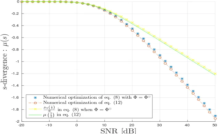
In Fig.5, we draw variouss-divergences:µ

1 2

,µ(s?),_N1µN

1 2

,_N1µN(s)ˆ . We can observe the

good agreement with the proposed theoretical results. Thes-divergence obtained by fixings= 1₂is accurate only at small SNR but degrades when SNR grows large.

-20 -10 0 10 20 30 40 50

SNR [dB]

-1.8 -1.6 -1.4 -1.2 -1 -0.8 -0.6 -0.4 -0.2 0

s-di

ve

rg

en

ce

:

µ

(

s

)

Numerical optimization of eq. (8) withΦ=Φ⊙

Numerical optimization of eq. (12)

µN(12)

N in eq. (8) whenΦ=Φ ⊙

µ!1₂"in eq. (12)

Figure 5.CPD scenario :s-divergencevsSNR in dB

In Fig. 6, we fixe SNR = 45 dB and draw s? obtained by eq. (14) versus values of c ∈ {10−6_{, 10}−5_{, 10}−4_{, 10}−3_{, 10}−2_{, 10}−1_{, 0.25, 0.5, 0.75, 0.9, 0.99} and the expression obtained by eq. (15).}

10-6 10-5

10-4 10-3

10-2 10-1

100

c

0.894 0.896 0.898 0.9 0.902 0.904

s

⋆

s⋆

= 1− 1

log(SNR)−1−1

−c

c log(1−c)

s⋆= 1 + 1

SNR−_log(1+SNR)1

Figure 6.CPD scenario:s?vsc , SNR=45 dB

For the TKD scenario, we follow the same methodology as above for CPD, Fig.7and Fig.8all agree with the analysis provided in section4.3.

-20 -10 0 10 20 30 40 50

SNR [dB]

0.5 0.55 0.6 0.65 0.7 0.75 0.8 0.85 0.9 0.95

s

⋆

Numerical optimization of eq. (7) for eq. (8)Φ=Φ⊗ Numerical optimization of eq. (16)

Analytical expression eq. (17)

-20 -10 0 10 20 30 40 50

SNR [dB]

-3 -2.5 -2 -1.5 -1 -0.5 0

s-di

ve

rg

en

ce

:

µ

(

s

)

Numerical optimization of eq. (8) withΦ=Φ⊗

Numerical optimization of eq. (16)

µN(12)

N in eq. (8) whenΦ=Φ

⊗

µ!1₂"in eq. (16)

Figure 8.TKD scenario :s-divergencevsSNR in dB

For TKD scenario, the mean square relative error is in mean of order−40 dB. So, we check numerically the consistency of the estimator of the optimals-value.

We can also notice that the convergence ofµN(s)

N towards its deterministic equivalentµ(s)in the

case TKD is faster than in the case CPD, since the dimension of matrixΦ⊗is 200.200.200×100.120.140 (N=2003) which is much larger than the dimension 6000×3000 ofΦ(N=6000).

6. Conclusion

In this work, we derived and studied the limit performance in terms of minimal Bayes’ error probability for the detection of high-dimensional random tensors using both the tools of Information Geometry (IG) and of Random Matrix Theory (RMT). The main results on Chernoff Bounds and Fisher Information are illustrated by Monte-Carlo simulations that corroborated our theoretical analysis.

For future work, we would like to study the rate of convergence and the fluctuation of the statistics µN(s)

N and ˆs. 7. Appendix

7.1. Proof of Lemma6

Thes-divergence in eq. (6) for the following binary hypothesis test (

H0 : y∼ N (0,Σ0), H1 : y∼ N (0,Σ1)

is given by [40]:

µN(s) =

1 2log

det(sΣ0+ (1−s)Σ1) [detΣ0]s[detΣ1]1−s

. (18)

Using the expressions of the covariance matricesΣ0andΣ1, the numerator in eq. (18) is given by

Nlogσ2+log det

and the two terms at its numerator are log[detΣ0]s =sNlogσ2and log[detΣ1]1−s = (1−s)

Nlogσ2+log det

SNR·ΦΦT_{+I .}

Using the above expressions,µN(s)is given by eq. (8).

7.2. Proof of Lemma7

If we notedΣ(SNR) = ∂Σ(x) ∂x

_x=SNRthen the following expression holds:

Σ(δSNR) =Σ(0) + (δSNR)·dΣ(0) =I+ (δSNR)·ΦΦT. Using the above expression, thes-divergence is given by

µN(s) = 1 −s

2 log det h

I+ (δSNR)·ΦΦT i

−1

2log det h

I+δSNR·(1−s)·ΦΦT i

Now, using eq. (8), and the following approximation:

1

Nlog det(I+xA) =

1

NTr log(I+xA)≈x·

1

NTrA− x2

2 · 1

NTrA 2

we obtain

µN(s)

N ≈(s−1)s·

(δSNR)2

2 ·

JF(0) N

where the Fisher information fory|δSNR∼ N(0,Σ(δSNR))is given by [34]:

JF(δSNR) =−E

∂2logp(y|δSNR) ∂(δSNR)2

= 1

2Tr{Σ(δSNR)

−1_dΣ(

δSNR)Σ(δSNR)−1dΣ(δSNR)} = 1

2Tr((I+ (δSNR)·ΦΦ

T₎−1_ΦΦT_(I+

δSNR)·ΦΦT)−1ΦΦT).

7.3. Proof of Theorem8

The first step of the proof is based on the derivation of an alternative expression ofµs(SNR)given

by eq. (18) involving the inverse of the covariance matricesΣ0andΣ1. Specifically, we have

µs(SNR) = 1

2log

(detΣ0)(detΣ1)det((1−s)Σ−01+sΣ

−1 1 ) [detΣ0]s[detΣ1]1−s

=−1

2log

det[(1−s)Σ−₀1+sΣ₁−1]−1 [detΣ0]1−s[detΣ1]s

. (19)

The second step is to derive a closed-form expression in the high SNR regime using the following

the approximation (see [7] for instance): x·ΦΦT+I−1 x≈1 Π⊥_Φ = IN−ΦΦ† whereΠ⊥_Φ is an

orthogonal projector such asΠ⊥_ΦΦ=0andΦ†= (ΦTΦ)−1ΦT. The numerator in eq. (19) is given by

h

(1−s)Σ−₀1+sΣ₁−1i−1 SNR≈1σ2

IN−sIN+sΠ⊥_Φ −1

=σ2

IN−sΦΦ† −1

AssΦΦ† is a rank-K projector matrix scaled by factors > 0, its eigen-spectrum is given by

s, . . . ,s | {z }

K

, 0, . . . , 0 | {z } N−K

. In addition, as the rank-Nidentity matrix and the scaled projectorsΦΦ† can be diagonalized in the same orthonormal basis matrix, then-th eigenvalue of the inverse of matrix

IN−sΦΦ†is given by

λn

IN−sΦΦ† −1

= 1

λn{IN} −sλn n

ΦΦ†o

=

( ₁

1−s, 1≤n≤K,

1, K+1≤n≤N

withs∈(0, 1). Using the above property, we obtain

log det[IN−sΦΦ†]−1

=log

N

∏

λn

IN−sΦΦ† −1

=−Klog(1−s). In addition, we have

log detSNR·ΦΦT+ISNR≈1Tr logSNR·ΦTΦ=K·log SNR+ K

∑

logλn

Finally, thanks to eq. (19), we have

µs(SNR) N

SNR1

≈ 1

2

K

N log(1−s) +s·log SNR+ s K

K

∑

logλn !

Finally, to obtains?in eq. (9), we solve ∂µs(SNR)

∂s =0.

7.4. Proof of Result9

Large random matrix theory allows to evaluate the asymptotic behavior ofµN(s)

N whenNq →+∞

for eachq=1, . . . ,Q,R→+∞in such a way that R_N1/_qq converge towards a non zero constant for each

q = 1, . . . ,Q. In other words, N1, . . . ,NQ converge towards+∞at the same rate (i.e. Nq

Np converge

towards a non zero constant for each(p,q)), andcR = NR converges towards a constantc > 0. In

this context, the empirical eigenvalue distribution of matrixΦ(Φ)Tconverges towards a relevant Marcenko-Pastur distribution. More precisely, we define the Marcenko-Pastur distributionνc(dλ)as the probability distribution given by

νc(dλ) =δ(λ) [1−c]++

q

λ−λ−c

λ+c −λ

2πλ 1[λ

−

c,λ+c](λ)dλ

whereλ−_c = (1− √

c)2andλ+_c = (1+ √

c)2. The Stieltjes transform ofνcdefined astc(z) =R_R+ νc

(dλ) λ−z is known to satisfy the equation

tc(z) =

−z+ c

1+tc(z) −1

Whenz∈_R−∗, i.e.z=−ρ, withρ>0, it is well known thattc(ρ)is given by

tc(−ρ) = 2

ρ−(1−c) + q

(ρ+λ−c)(ρ+λ+c )

(20)

It was established for the first time in [38] that if Xrepresents a K×Prandom matrix with zero mean and _K1 variance i.i.d. entries, and if(λk)k=1,...,Krepresent the eigenvalues ofXXTarranged in

decreasing order, then the so-called empirical eigenvalue distribution ofXXTdefined as _K1∑K_k=1δ(λ− λk)converges weakly almost surely towardsνcin the asymptotic regime whereK→+∞,P→+∞,

P

K →c. In particular, for each continuous function f(λ), it holds that

1

K K

∑

f(λk) a.s −→

Z

R+

f(λ)νc(dλ). (21)

In practice, this result means that ifKandPare large enough, then the histogram of the eigenvalues of each realization ofXXTtends to accumulate around the graph of the probability density ofνc.

The columns(φ_r)r=1,...,R ofΦ are vectors(φr(Q)⊗. . .⊗φr(1))r=1,...,R. These vectors are mutually

independent, identically distributed, and satisfyE(φ_rφT_r) = I_NN. However, the elements ofΦare not mutually independent because the components of each columnφ_rare not independent. In the asymptotic regime considered in this paper, the results of [44] (see also [3]) allow to establish that the empirical eigenvalue distribution ofΦ(Φ)Tstill converges almost surely towardsνc, where we

recall that _NR →c. Using (21) forf(λ) =log(1+λ/ρ)as well as a well-known formula that allows to expressR

R+log(1+λ/ρ)νc(dλ)in terms oftc(−ρ)given by (20) (see e.g. [50]), we obtain the result. 7.5. Proof of Result14

We haveu(x)c≈1 1 x+

q

(1_x+1)2₌ 2

x+1 andu(x) + (1−c) c1

≈ 21_x+1,u(x)−(1−c)c≈1 2 x,

u(x)2−(1−c)2c≈1 4 x

1 x+1

. Using the above first-order approximations, eq. (13) is

Ψc1(x) 1 ≈c· x

1+x+clog(1+x)−c x

1+x =clog(1+x).

Using the above approximation and eq. (12), we obtain Result14.

7.6. Proof of Result15

We first denoteλ(₁q)≥λ(₂q)≥...≥λ(nqq)≥...≥λ (q)

Nq the eigenvalues ofΦ

(q)_(Φ(q)₎T_{, 1≤n} q ≤Nq,

for 1≤ q≤ Q. We can notice that the eigenvalues ofΦ⊗(Φ⊗)Tareλ(n1₁)· · ·λ(nQ_Q). Moreover, in the

asymptotic regime, whereMq →+∞,Nq →+∞such that M_Nqq →cq, 0<cq <1, for all 1≤q≤Q, we

have thatλ(nqq)=0 ifMq+1≤nq ≤Nqand the empirical distribution of the eigenvalues(λ (q)

nq)1≤nq≤Mq

behaves as Marchenko-Pastur distributionsνcq of parameters(cq, 1). Recalling thatM = M1...MQ,

N=N1...NQ, we obtain immediately that

1

Nlog det

SNR·Φ⊗(Φ⊗)T+I= 1 N

N1

∑

...

NQ

∑

logSNR·λ(n11)· · ·λ

(Q)

nQ +1

= M N 1 M M1

∑

...

M_Q

∑

logSNR·λ(n11)· · ·λ

(Q)

nQ +1

and that

1

M M1

∑

...

MQ

∑

logSNR·λ(n11)· · ·λ

(Q)

nQ +1

_a.s −→

Z +∞

0 ...

Z +∞

0 log(1+SNR·λ1...λQ)dνc1(λ1)...dνcQ(λQ)

Similarly, we have that

1

Mlog det

SNR·(1−s)Φ⊗(Φ⊗)T+I−→a.s

Z +∞

0 ...

Z +∞

0 log(1+SNR·(1−s)λ1...λQ)dνc1(λ1)...dνcQ(λQ)

We obtain easily result15.

Acknowledgments:The authors would like to thank Professor Philippe Loubaton (UPEM, France) for the fruitful discussions.

References

1. M. Abramowitz, I. A. Stegun (Eds.). "Elliptic Integrals." Ch. 17 inHandbook of Mathematical Functions with Formulas, Graphs, and Mathematical Tables, 9th printing, New York Dover Publications, pp. 587-607, 1972. 2. S. M. Ali, S. D. Silvey,A General Class of Coefficients of Divergence of One Distribution from Another, Journal of

the Royal Statistical Society. Series B (Methodological) Vol. 28, No. 1 (1966), pp. 131-142

3. A. Ambainis, A. W. Harrow and M. B. Hastings,Random matrix theory: extending random matrix theory to mixtures of random product states, Commun. Math. Phys., vol. 310, no. 1, pp. 25-74 (2012).

4. R. Badeau, G. Richard and B. David,Fast and stable YAST algorithm for principal and minor subspace tracking. IEEE J SP, IEEE, 2008, 56 (8), pp.3437-3446.

5. Z. D. Bai, J. W. Silverstein. Spectral analysis of large dimensional random matrices. Springer Series in Statistics, 2nd edition, 2010.

6. J. Baik, J. Silverstein,Eigenvalues of large sample covariance matrices of spiked population models, Journal of Multivariate Analysis, Volume 97, Issue 6, July 2006, Pages 1382-1408

7. R. T. Behrens, L. L. Scharf,Signal processing applications of oblique projection operators. IEEE Transactions on Signal Processing, Vol 42, pp 1413-1424, 1994.

8. O. Besson , L.L. Scharf, "CFAR matched direction detector",IEEE Transactions on Signal Processing, Volume: 54, Issue: 7, July 2006.

9. P. Bianchi, M. Debbah, M. Maida, and J. Najim,Performance of Statistical Tests for Source Detection using Random Matrix Theory, IEEE Trans. on Information Theory, vol. 57, no. 4, pp. 2400-2419, April 2011.

10. M. Boizard, G. Ginolhac, F. Pascal, and P. Forster, Low-rank filter and detector for multidimensional data based on an alternative unfolding HOSVD: application to polarimetric STAP. EURASIP Journal on Advances in Signal Processing, SpringerOpen, 2014, 2014, pp.119.

11. G. Bouleux and R .Boyer,Sparse-Based Estimation Performance for Partially Known Overcomplete Large-Systems, Signal Processing, Volume 139, October 2017, pp. 70-74.

12. R. Boyer and R. Badeau. Adaptive multilinear SVD for structured tensors. IEEE International Conference on Acoustics, Speech, and Signal Processing (ICASSP’06), 2006, Toulouse, France. 2006.

13. R. Boyer and C. DelphaRelative-entropy based beamforming for secret key transmission, IEEE 7th Sensor Array and Multichannel Signal Processing Workshop (SAM), 2012.

14. R. Boyer, R. Couillet, B-H. Fleury, and P.Larzabal,Large-System Estimation Performance in Noisy Compressed Sensing with Random Support - a Bayesian Analysis, IEEE Transactions on Signal Processing, Volume 64, No. 21, 2016, pp. 5525-5535.

15. R. Boyer and P. Loubaton,Large deviation analysis of the cpd detection problem based on random tensor theory, European Association for Signal Processing (EUSIPCO), 2017.

16. R. Boyer and F. Nielsen,Information Geometry Metric for Random Signal Detection in Large Random Sensing Systems, IEEE International Conference on Acoustics, Speech, and Signal Processing, (ICASSP), 2017. 17. Y. Cheng, X. Hua, H. Wang, Y. Qin and X. Li,The Geometry of Signal Detection with Applications to Radar Signal

18. S. P. Chepuri and G. Leus,Sparse sensing for distributed Gaussian detection,IEEE International Conference on Acoustics, Speech and Signal Processing (ICASSP), 2015.

19. H. Chernoff,A Measure of Asymptotic Efficiency for Tests of a Hypothesis Based on the sum of Observations, Ann. Math. Statist. Volume 23, Number 4 (1952), 493-507.

20. A. Cichocki, D. Mandic, L. De Lathauwer, G. Zhou, Q. Zhao, C. Caiafa, and H. A. Phan,Tensor decompositions for signal processing applications: From two-way to multiway component analysis,IEEE Signal Processing Magazine, vol. 32, no. 2, pp. 145-163, 2015.

21. P. Comon, J. T. Berge, L. De Lathauwer and J. Castaing,Generic and Typical Ranks of Multi-Way Arrays, Linear Algebra and its Applications, Elsevier, 2009, 430 (11), pp.2997-3007.

22. P. Comon, X. Luciani and A. L. F. de Almeida,Tensor decompositions, alternating least squares and other tales, Journal of Chemometrics, 2009.

23. P. Comon ,Tensors : A brief introduction, IEEE Signal Processing Magazine , Volume: 31, Issue: 3, May 2014. 24. T. M. Cover and J. A. Thomas,Elements of information theory, John Wiley & Sons, 2012

25. L. De Lathauwer, B. D. Moor, and J. Vandewalle,A Multilinear Singular Value Decomposition, SIAM Journal on Matrix Analysis and Applications, 2000, Vol. 21, No. 4 : pp. 1253-1278

26. L. De Lathauwer,A survey of tensor methods, IEEE International Symposium on Circuits and Systems, 2009. ISCAS 2009.

27. N. Duy Tran, R. Boyer, S. Marcos, and P. Larzabal,Angular resolution limit for array processing: Estimation and information theory approaches, Proceedings of the 20th European Signal Processing Conference (EUSIPCO), 2012.

28. C. Eckart and G. Young,The approximation of one matrix by another of lower rank, Psychometrika, September 1936, Volume 1, Issue 3, pp 211–218.

29. V. L. Girko,Theory of random determinants, Kluwer Academic Publishers,1990.

30. J. H. D. M. Goulart, M. Boizard, R. Boyer, G. Favier and P. Comon,Tensor CP Decomposition with Structured Factor Matrices: Algorithms and Performance, IEEE Journal of Selected Topics in Signal Processing, IEEE, 2016, 10 (4), pp.757-769.

31. E. Grossi and M. Lops,Space-time code design for MIMO detection based on Kullback-Leibler divergence, IEEE Trans. Inf. Theory, vol. 58, no. 6, pp. 3989-4004, Jun. 2012.

32. T. Kailath,The Divergence and Bhattacharyya Distance Measures in Signal Selection. IEEE Transactions on Communication Technology, 15, 52-60, 1967.

33. G. Katz, P. Piantanida, R. Couillet and M. Debbah,Joint estimation and detection against independence, Annual Conference on Communication Control and Computing (Allerton), pp. 1220-1227 Sept 2014.

34. S. M. Kay,Fundamentals of statistical signal processing, Volume II: Detection theory, PTR Prentice-Hall,Englewood Cliffs, NJ, 1993.

35. Y. Lee, Y. Sung,Generalized Chernoff Information for Mismatched Bayesian Detection and Its Application to Energy Detection, IEEE Signal Processing Letters, Volume: 19, Issue: 11, Nov. 2012.

36. P. Loubaton and P. Vallet,Almost Sure Localization of the Eigenvalues in a Gaussian Information Plus Noise Model. Application to the Spiked Models. Electron. J. Probab. Volume 16 (2011), paper no. 70, 1934-1959.

37. A. Lytova,Central Limit Theorem for Linear Eigenvalue Statistics for a Tensor Product Version of Sample Covariance Matrices, Journal of Theoretical Probability, 2017.

38. V. A. Marchenko and L. A. Pastur,Distribution of eigenvalues for some sets of random matrices, Mat. Sb. (N.S.), 72(114):4, 507–536, 1967.

39. X.Mestre,Improved Estimation of Eigenvalues and Eigenvectors of Covariance Matrices Using Their Sample Estimates, IEEE Transactions on Information Theory, Volume: 54, Issue: 11, Nov. 2008.

40. F. Nielsen,Chernoff information of exponential families. CoRR 2011, abs/1102.2684.

41. F. Nielsen,An information-geometric characterization of Chernoff information, IEEE Signal Processing Letters, vol. 20, no. 3, pp.269-272, 2013.

42. F. Nielsen, Hypothesis testing, information divergence and computational geometry, Geometric Science of Information, Springer, 2013, pp. 241-248

44. A. Pajor, L. A. Pastur, On the Limiting Empirical Measure of the sum of rank one matrices with log-concave distribution, Studia Math, 195 (2009), pp: 11-29.

45. S. Sen, A. Nehorai,Sparsity-Based Multi-Target Tracking Using OFDM Radar, IEEE Transactions on Signal Processing, Volume: 59, Issue: 4, April 2011 .

46. J. W. Silverstein, P. L. Combettes,Signal detection via spectral theory of large dimensional random matrices. IEEE Transactions on Signal Processing , Volume. 40. No. 8. August 1992.

47. S. Sinanovic, D. H. Johnson,Toward a theory of information processing, Signal Processing, vol. 87, no. 6, pp. 1326-1344, 2007.

48. G. Tang, A. Nehorai,Performance Analysis for Sparse Support Recovery, IEEE Transactions on Information Theory, Volume: 56, Issue: 3, March 2010.

49. L. R. Tucker, Some mathematical notes on three-mode factor analysis, Psychometrika (1966) 31: 279. https://doi.org/10.1007/BF02289464.

50. A. M. Tulino, S. Verdu, Random Matrix Theory and Wireless Communications, Hanover, MA, USA: Now Publishers Inc., Jun. 2004, vol. 1, no. 1.

51. D. Voiculescu,Limit laws for random matrices and free products, Invent. Math. 104 (1991) 201.

52. E. P. Wigner,On the statistical distribution of the widths and spacings of nuclear resonance levels, Proc. Cam. Phil. Soc. 47 (1951) 790.