Article
1
Sensitivity of Different Parameterizations on
2
Simulation of Tropical Cyclone Durian over the
3
South China Sea using Weather Research and
4
Forecasting (WRF) model
5
Worachat Wannawong 1,*, Donghai Wang 1, Yu Zhang 1 and Chaiwat Ekkawatpanit 2
6
1 School of Atmospheric Sciences, Sun Yat-sen University, Guangzhou 510275, China
7
2 Department of Civil Engineering, Faculty of Engineering, King Mongkut's University of Technology
8
Thonburi, Bangkok 10140, Thailand
9
* Correspondence: [email protected]; Tel.: +86-131-4311-3438
10
11
Abstract: Typhoon Durian forming over the Western North Pacific Ocean and entering into the
12
South China Sea (SCS), caused extreme and widespread damages in 2006. In this research,
13
sensitivity analyses on different physical parameterization schemes of the Weather Research and
14
Forecasting Atmospheric Model (WRF-ATM) have been utilized to study typhoon Durian. Model
15
accuracy and performance testing were investigated with different initial conditions during the
16
tropical cyclone simulation in the SCS. The initial and boundary conditions (IBCs) for all
17
experiments were derived from the European Centre for Medium Range Weather Forecasts
18
(ECMWF), Re-Analysis Interim (ERAI), and the National Centers for Environmental Prediction
19
(NCEP) with Final (FNL) analysis data compiled through the WRF-ATM model. The sensitivity
20
analysis results indicated a major improvement for the cumulus scheme by using the
21
Grell-Devenyi scheme along with the PBL scheme of Yonsei University, mixed-phase microphysics
22
scheme of the WRF Single Moment 5-class and IBCs for ECMWF-ERAI of TC simulation under the
23
context of Wind-Pressure Relationships. This predicted better track and intensity comparing with
24
these of the Joint Typhoon Warning Center. The results revealed that the TC track and intensity
25
were well simulated by the WSM5-GD combination for the WRF-ATM model with an intensity
26
error of 1.69 hPa for minimum surface level pressure, maximum wind speed of 1.83 knots and
27
average track error of 25 km in 72 hours. The simulations showed that the potential track and
28
intensity error decreased with the delayed IBCs, suggesting that the model simulation is more
29
dependable when the coast is approached by the TC.
30
Keywords: Typhoon Durian; Tropical cyclone; Wind-Pressure Relationships; South China Sea;
31
Sensitivity analysis; WRF
32
33
1. Introduction
34
Severe Tropical Cyclones (TC) in the Western North Pacific (WNP) Ocean and the South China
35
Sea (SCS) are one of the most destructive weather phenomena. Heavy rainfall, flooding, landslides,
36
strong winds, low pressure, high waves, and storm surge are the major hazards associated with TC
37
activities [1–3]. Loss of life and livelihoods caused by intense cyclones could be substantially
38
reduced by appropriate mitigation strategies including accurate and long lead forecasting. Recently,
39
the model studies as well as the Weather Research and Forecasting Atmospheric Model (WRF-ATM)
40
have been used to examine the TC mechanism induced by the atmospheric and oceanic conditions,
41
e.g., the Sea Surface Temperature (SST) and heat fluxed changes at the surface over the WNP Ocean
42
and the SCS [4]. The WRF-ATM model is the regional Numerical Weather Prediction (NWP) model
43
which can be used to predict the meteorological phenomena - including the TC potential track and
44
its intensity. It is one of the most well-known numerical weather prediction models in mesoscale
45
simulation systems. In addition, the WRF-ATM model is not only able to be used for simulation of
46
real and ideal cases, but also in providing various physical parameterizations for a theoretical basis
47
to study the physical process and integration with multiple models as in a fully coupled model [5].
48
This model uses initial boundary conditions (IBCs) to solve the dynamical atmospheric and
49
thermodynamic equations with the assumptions of some physics options. The model simulations for
50
the scale analysis as in the mesoscale predictions are highly sensitive to the physical
51
parameterizations used in model forecasting with complex topography, especially in the SCS.
52
Cumulus convection and boundary layer physics play an important role in the development and
53
intensification of TC prediction. Although parameterization schemes have some limitations on the
54
prediction of the TC track and its intensity, they play a very crucial role in weather event
55
simulations.
56
The sensitivity study is, therefore, an approach to identify the impact of different physical
57
parameterizations and IBCs on the TC track and intensity simulation under the Wind–Pressure
58
Relationships (WPRs) with a smooth curve for the statistical validation of model simulations and
59
observation. In recent years, Islam et al. [6] studied the sensitivity of model physical
60
parameterizations on simulation of super typhoon Haiyan 2013 over the WNP Ocean by using two
61
different datasets from the European Centre for Medium Range Weather Forecasts (ECMWF),
62
Re-Analysis Interim (ERAI) and the National Centers for Environmental Prediction (NCEP) Global
63
Forecast System (GFS) data. Their study suggested that the best choice of physical combination and
64
parameterization for the typhoon Haiyan case study is in the WNP Ocean under the WPRs for the
65
comparison of model simulations and observation. The simulation results were compared with the
66
best track obtained from the Joint Typhoon Warning Centre (JTWC) based on the criteria of Root
67
Mean Square Error (RMSE). It was found that the lowest intensity error was 4.21 hPa for Minimum
68
Surface Level Pressure (MSLP), Maximum wind speed (Vmax) was 3.26 knots and average track error
69
was 87.33 km in 48 hours forecasted by using the WRF single moment 6-class (WSM6) for
70
microphysics scheme with the Quasi-Normal Scale Elimination (QNSE) for the Planetary Boundary
71
Layer (PBL) combination. Other sensitivity studies related to the WRF-ATM physical
72
parameterizations can be found in Srivastava et al. [7] and Mooney et al. [8].
73
For the study cases with the performance testing, Wang [9] presented that a high-resolution
74
model results showed its performance for TC simulations. A high-resolution experiment using
75
nested grids of 15-km and 5-km grid spacing with 183×195 and 267×273 grid points, respectively,
76
had been set up in order to better investigate the impact of the vortex relocation on the intensity
77
forecast. A better definition of the initial vortex was found as a major reason for the TC track and its
78
intensity improvements for a short-term prediction. For long-term simulations, the WRF-ATM
79
model with TC simulation results was also widely used in the WNP Ocean [4].
80
In this research, super typhoon Durian (2006) has been used as a case study. Its track spanned
81
15 days without a decrease of TC’s primary energy after passing the Philippines. It continued
82
heading toward the SCS to the Gulf of Thailand (GoT) and the onwards to the Bay of Bengal (BoB). It
83
was also classified as one of two typhoons showing strong power crossing the North-West Pacific
84
Ocean into the BoB. In this work, TC activities including wind and pressure changes have been
85
investigated by using the SST update under the surrounding oceanic environments, different
86
physical parameterizations, and IBCs. The impact on TC position tracking and intensity were also
87
studied. In addition, to our knowledge, the sensitivity analysis of different parameterizations on
88
super typhoon Durian using WRF-ATM model has not been studied. The present work, therefore,
89
aimed at investigating for the sensitivity of physical parameterization schemes of super typhoon
90
Durian over the SCS. The model accuracy and performance testing were also presented by using the
91
WPRs of the WRF-ATM model simulations and best-track datasets.
2. Description of Typhoon, Model Configuration and Analysis
94
2.1. A Brief Overview of Super Typhoon Durian
95
Super typhoon Durian (category 4) was formed as a tropical depression at 1200 UTC 24
96
November 2006 which was reported by the JTWC. The pre-Durian disturbance was tracked at the
97
initial location of 6.1° N, 149.8° E. The tropical depression intensity slowly intensified and moved
98
west to west-northwestward with Vmax of 15 knots and MSLP of 1006 hPa. Its intensity was upgraded
99
from tropical depression to tropical storm at 0600 UTC on 26 November with Vmax of 35 knots and
100
MSLP of 997 hPa at the location of 9.7° N, 142.8° E. A few days later, it developed rapidly, achieving
101
typhoon strength and acquiring the name Durian at 1200 UTC on 28 November with Vmax of 65 knots
102
and MSLP of 976 hPa at the location of 12.1° N, 131.6° E according to the JTWC records. Its intensity
103
was then upgraded to a category 4 Super Typhoon at 1200 UTC on 29 November and 0000 UTC on
104
30 November. In this study, the model experiments and their simulations were used to validate with
105
the JTWC best-track data. The model simulations were conducted between 0000 UTC 2 December to
106
0000 UTC 5 December 2006 covering a period of Durian intensity in the SCS as shown in Figure 1.
107
108
109
Figure 1. Study domains (D01 and D02) of WRF-ATM model, associated with JTWC best track data from 0000
110
UTC 2 December to 0000 UTC 5 December 2006. The daily intervals of track locations are shown in the pink
111
squares.
112
2.2. Model Description and Configuration
113
The WRF-ATM model version 3.7.1 [10] was applied in this study. This model version is part of
114
a full package of coupled modeling systems [5]. In this work, the WRF-ATM model was built with
115
the Automated Tropical Cyclone Forecasting (ATCF) two-way vortex-following the moving nested
116
grid domains for a short-term simulation. The study domain was configured at the center point of
117
10° N, 112°E (latitude-longitude). A two-way nesting was employed or the interaction between
118
outer and inner domains as shown in Figure 1. The parent domain has been set up for 219×174 grid
119
points with a 15-km grid spacing, while the child domain has been set up for 180×180 grid points
120
with a 5-km grid spacing as shown in Table 1. The NCEP-Final (FNL) reanalysis and ECMWF-ERAI
121
global model datasets were used to provide the IBCs with 30 terrain following and the top of model
122
at 50 hPa for both domains in the WRF-ATM experimental simulations. The model studies have been
123
illustrated by the different IBCs global model datasets with physics options combination. The model
124
results with sensitivity analysis by physical parameterizations and performance testing have been
125
compared with the JTWC best-track data under the WPRs (Table 2).
Table 1. Model configuration of WRF-ATM
127
Model setup Information
Grid points Outer domain: 221x174 (D01)
Inner domain: 180x180 (D02)
Horizontal resolution Outer domain: 15 km (D01)
Inner domain : 5 km (D02) Vertical resolution 30 layers;
Model top set to 50 hPa
Centered domain 11oN, 113oE
Time step 90 sec
Map projection
IC/BCs
Mercator
1. ECMWF-ERAI:
1.1 6-h time interval by ERAI
1.2 Daily ERAI-SST averaged from ECMWF
1.3 0.75°×0.75° horizontal and 61 vertical grid resolutions 2. NCEP-FNL:
2.1 6-h time interval by FNL
2.2 Daily RTG-SST updated from NCEP/NOAA
2.3 1.0°×1.0° horizontal and 27 vertical grid resolutions Simulation/Spin-up
periods
3. ECMWF-ERAI:
3.1 0000 UTC 01 Dec–0000 UTC 06 Dec/1 day 3.2 1200 UTC 01 Dec–0000 UTC 06 Dec/0.5 days 4. NCEP-FNL:
4.1 0000 UTC 01 Dec–0000 UTC 06 Dec/1 day 4.2 1200 UTC 30 Nov–0000 UTC 06 Dec/1.5 days
128
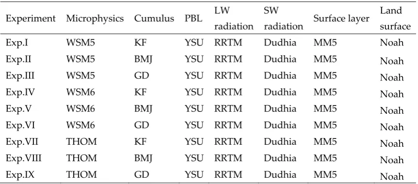
Table 2. Differences of physical parameterizations of WRF-ATM model sensitivity analysis
129
Experiment Microphysics Cumulus PBL LW radiation
SW
radiation Surface layer Land surface
Exp.I WSM5 KF YSU RRTM Dudhia MM5 Noah
Exp.II WSM5 BMJ YSU RRTM Dudhia MM5 Noah
Exp.III WSM5 GD YSU RRTM Dudhia MM5 Noah
Exp.IV WSM6 KF YSU RRTM Dudhia MM5 Noah
Exp.V WSM6 BMJ YSU RRTM Dudhia MM5 Noah
Exp.VI WSM6 GD YSU RRTM Dudhia MM5 Noah
Exp.VII THOM KF YSU RRTM Dudhia MM5 Noah
Exp.VIII THOM BMJ YSU RRTM Dudhia MM5 Noah
Exp.IX THOM GD YSU RRTM Dudhia MM5 Noah
130
2.3. Initial and Lateral Boundary Conditions
132
For the IBCs, the WRF-ATM model is used to downscale from the ECMWF-ERAI global
133
scale-reanalysis data with 0.75°×0.75° horizontal and 61 vertical grids to the regional grid domains of
134
all model experiments at 15 and 5 km resolutions. The main feature of the ECMWF-ERAI global
135
model has been improved by the 4DVAR data assimilation, while the 3DVAR data assimilation has
136
been using for the NCEP-FNL model components and analysis. The ECMWF-ERAI time range
137
covers from 1979 to present and the SST has also been included, whereas the NCEP-FNL models
138
time range covers from 1999 to present. The resolution of ECMWF-ERAI meteorological grid level in
139
horizontal and vertical coordinates are finer than the NCEP-FNL reanalysis data with 1.0°×1.0°
140
horizontal and 27 vertical grids. The model recommendation for the WRF-ATM model modification
141
with the NCEP-FNL model data has been updated by the Real-Time Global (RTG)-SST with the
142
0.5°×0.5° horizontal grids.
143
In this study, the model configuration has been applied for two-way vortex-following moving
144
nested grids and modeled feedback between both domains with the TC model experiments and
145
numerical simulations. The two-way nesting was available for the model interaction between both
146
domains with the ATCF.
147
Figure 1 illustrates the D01-outer and D02-inner domains with parent and child domains, which
148
covered some parts of the Indochinese Peninsula (IP) including the SCS and GoT. For all model
149
experiments, both ECMWF-ERAI and NCEP-FNL datasets were available as 6-hour reanalysis data,
150
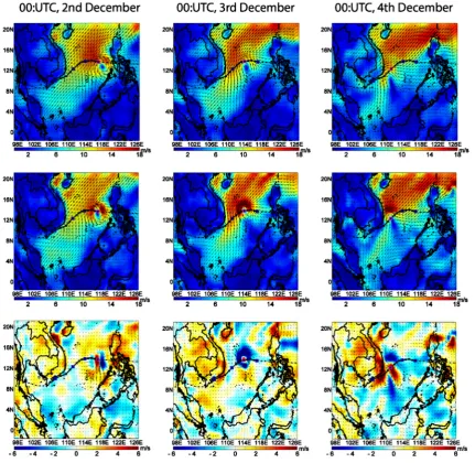
which has been used for the WRF-ATM IBCs model. Figures 2–4 show the sample initial datasets
151
and differences of ECMWF-ERAI and NCEP-FNL for wind, sea level pressure and SST fields from
152
0000 UTC 2 December to 0000 UTC 4 December 2006. This data has been used as the initial data for
153
the model integration of nine experimental designs with different IBCs and model spin-up periods
154
for 36 case studies. It was performed without observation assimilation as shown in Tables 1 and 2.
155
The model consideration began at 0000 UTC 2 December 2006, and continued until 0000 UTC 5
156
December 2006 with different spin-up times. The first experiment with 24 hour (1 day) forecast was
157
considered for the model spin-up time. The second experiment for different spin-up running with 12
158
hours (0.5 days) and 36 hours (1.5 days) forecasts were also mainly discussed by the average daily
159
weather considerations. Another model experiment of the WRF model with the differences of ERAI
160
and FNL IBCs for 1.5 and 0.5 day spin-up periods were not presented here.
162
Figure 2. Sample IBCs of wind fields (m/s) at the 10-meter height level. ECMWF-ERAI (top row), NCEP-FNL
163
(middle row), and difference of both IBCs (bottom row) from 0000 UTC 2 December to 0000 UTC 4 December
164
2006.
165
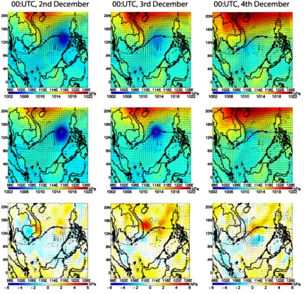
Figure 3. As in Figure 2, but for surface level pressure (hPa).
167
169
Figure 4. As in Figure 3, but for sea surface temperature (°C).
170
2.4. Physical Parameterizations of Model Simulation
171
The impact of model physics options on TC simulations was described in this study. These
172
physical parameterizations and their combinations were conducted for two major physics schemes -
173
Microphysics (MP) and Cumulus (Cu) parameterizations with specific Planetary Boundary Layer
174
(PBL) for nine experiments (Experiment I to Experiment IX). The best choice of physics options was
175
investigated by using both IBCs for the model accuracy and performance testing as summarized in
176
Table 2.
177
For the first sensitivity analysis, the WRF-ATM experimental models were designed for three
178
different combinations to study the differences of MP and Cu schemes by the TC simulations. The
179
MP schemes provided the atmospheric heat and moisture tendencies with the vertical flux of cloud,
180
precipitation and sedimentation processes of hydrometeors [11]. The MP scheme determinations
181
widely used in the WRF-ATM model community included the WRF Single Moment 5-class (WSM5),
182
WRF Single Moment 6-class (WSM6), and Thompson (THOM) schemes [10]. The WSM5 scheme was
183
updated from the original scheme, viz., the WRF Single Moment 3-class (WSM3). It was also allowed
184
for the mixed-phase processes of cloud water/ice, rain, snow and super-cooled water. The WSM5
185
scheme was chosen after some initial tests showing that this scheme agreed well with the more
186
complicated MP schemes.
For the newly issued conceptual framework of WSM, graupel was introduced as another
188
variable which measured a new combined snow/graupel fall speed in the WSM6 scheme, while the
189
ice number concentration still followed the concept of WSM3 and WSM5 schemes [12]. In addition,
190
the new THOM scheme [13] was applied to study the impacts of MP schemes in the final application
191
of this section. The generalized gamma distribution shape of each hydrometeor species by the new
192
THOM scheme distributed the new snow parameterization depending upon both ice/water content
193
and temperature. A summary of overall analysis, the MP schemes have been accompanied by the
194
Yonsei University (YSU) PBL scheme [14]. The MM5 surface layer, Noah Land Surface Model (LSM),
195
Long-Rapid Radiative Transfer Model (RRTM) and short wave radiation schemes were also required
196
[15] as described in Table 2.
197
It was found that the Cu schemes were not kept fixed (Table 2). The model experimental
198
simulations were applied for three Cu-schemes. The first Cu-scheme was started by the Kain-Fritsch
199
(KF) [16]. For deep tropical convection, the Betts-Miller-Janjic (BMJ) scheme provides the
200
characteristic profiles of temperature and moisture. The deep convection profiles are proportional to
201
the entropy change, precipitation, mean cloud temperature and efficiency, while the shallow
202
convection moisture profile requires a non-negative change of entropy [17]. For the last Cu scheme,
203
the Grell-Devenyi (GD) scheme [18] has been simplified for the modified quasi-equilibrium
204
assumption and equilibrium in the mass flux scheme. The GD scheme is based on the Convective
205
Available Potential Energy (CAPE), low-level vertical velocity and moisture convergence, thickness
206
of the capping inversion and the dependence of the downdraft on the precipitation efficiency,
207
leading to more variability in the ensemble spread. The ensemble spread is introduced by effective
208
multiple Cu schemes and variants which run within each grid box. It is also averaged to provide
209
feedback to the model.
210
However, the TC sensitivity analysis only examined YSU for the PBL physical
211
parameterizations and also kept fixed for the Rapid Radiative Transfer Model (RRTM) Long Wave
212
(LW) radiation [19], Dudhia shortwave radiation schemes [20], MM5 similarity surface layer, and the
213
Noah Land Surface Model [15].
214
2.5. Statistical Verification and Operational Agency Equations
215
In this research, the TC experiments were simulated in nine physical combinations with two
216
different IBCs and spin-up periods by the ATCF two-way vortex-following moving nested grid
217
domains for the sensitivity study and analysis as shown in Tables 1 and 2 for 36 case studies. These
218
studies were classified by the intensity of Vmax, MSLP and potential track area under the WPRs
219
through the WRF-ATM model experiments. In this section, the main state was to validate the model
220
simulations with the JTWC best-track data. The TC model experiments were also reanalyzed by
221
exhibiting a smooth descending trend of Vmax and MSLP with the operational agency equations to
222
represent the real state of the simulation variables. Three statistical indexes, which wereBias, Root
223
Mean Squared Error (RMSE), andStandard Deviation Error (STDE), with five operational agency
224
equations (Opa.I–Opa.V) were utilized for model accuracy evaluation and performance testing.
225
Equations used by the operational center agencies are as follows.
226
The equation for the National Hurricane Center/Tropical Prediction Center and the Central
227
Pacific Hurricane Center/Operational agency (Opa.I) has been applied from the Dvorak [21]
228
equation:
229
MSLP = 1,021.36 0.36V
−
max−
(
V
max/
20 16
.
)
2 (1)230
The equation used by the Regional Specialized Meteorological Center (RSMC)/Operational
231
agency (Opa.II) in Tokyo has been adapted from the Knaff and Zehr [22] equation or Koba equation:
232
MSLP = 6.22 0.58V
−
max−
(
V
max/
31 62 +1,010
.
)
2 (2)The RSMC La Reunion Island, RSMC Fiji, Perth Tropical Cyclone Center, and Joint Typhoon
234
Warning Center (JTWC)/Operational agency (Opa.III) have followed the Atkinson and Holliday [23]
235
equation:
236
MSLP =
−
(
V
max/ .
6 7
)
1 553.+1,010
(3)237
The Darwin Center/Operational agency (Opa.IV) applied the Love and Murphy [22] equation:
238
MSLP = 6.37 0.54V
−
max−
(
V
max/
43 03 +1,010
.
)
2 (4)239
The equation used by the Brisbane Center/Operational agency (Opa.V) is applied from the
240
Crane [22] equation:
241
MSLP = 5.82 0.50V
−
max−
(
V
max/
22 20 +1,010
.
)
2 (5)242
where Vmax is the maximum surface wind (in knots) and MSLP is the minimum surface level
243
pressure (in hPa).
244
3. Interpretation of Model Simulation Results
245
The TC potential track and its intensity have been considered to be the most important and
246
challenging contents for the NWP systems. The model accuracy of TC tracking is most crucial to
247
examine the geographical location where actual damages due to TC intensity such as strong wind
248
associated with low pressure. Misinformation from the TC center by the NWP system would
249
produce inaccurate TC tracking and its intensity with circulation at the actual location on land and
250
sea. Therefore, the TC simulation testing through WRF–ATM model experiments and its sensitivity
251
analysis are essential to locate areas of TC intensities in the SCS. In section 3.1, the impact of different
252
physical parameterization schemes for the TC predictions is discussed.
253
3.1. Impact of Microphysics and Cumulus Combination Schemes
254
The TC track and its intensity prediction of three KF, BMJ, and GD Cu-convective schemes with
255
combination of three WSM5, WSM6 and THOM MP-schemes are discussed in this section. Figures 5
256
and 6 show nine-experimental designs of TC Durian simulations of location tracking (top panel) and
257
its intensity as Vmax (middle panel) and MSLP (bottom panel) associated with the JTWC observed
258
track, different IBCs and spin-up periods.
260
Figure 5. Time series of ECMWF-ERAI (left column) and NCEP-FNL IBCs (right column) by using WRF-ATM
261
model simulations, associated with JTWC best-track data. TC potential track simulations (top row), Vmax (knots)
262
(middle row), and MSLP (hPa) (bottom row). The daily intervals of track locations are shown in the pink
263
squares from 0000 UTC 2 December to 0000 UTC 5 December 2006 (1 day spin-up time).
264
266
Figure 6. As in Figure 5, but for different model spin-up times, 0.5 days for ECMWF-ERAI (left panel) and 1.5
267
days for NCEP-FNL IBCs (right panel).
268
The GD combinations showed better TC location tracking with a group of three MP schemes
269
comparing with the JTWC best-track data, especially for a physical combination of WSM5
270
MP-scheme (Experiment III) by using the ECMWF-ERAI IBCs of one day spin-up period on a
271
specific model driving. However, the GD scheme with a combination of three MP schemes fails at
272
the strong influence of upwelling area with high SST variability [24,25] as in the South-eastern Coast
273
of Vietnam (SCOV). The vector displacement error for TC simulated tracks with above stated
274
schemes are demonstrated in Tables 3 and 4, as well as those two figures in the top panel of Figures 5
275
and 6.
276
277
Table 3. Daily average track errors (in km) of model experiments derived by ECMWF-ERAI IBCs with different
279
simulation/spin-up periods, associated with JTWC best-track achieves.
280
Experiment
1 day spin-up period 0.5 days spin-up period
Day 1 Day 2 Day 3 Avg. Day 1 Day 2 Day 3 Avg.
Exp.I 93 117 229 146.3 27 71 127 75.1
Exp.II 76 66 66 69.3 54 82 72 69.1
Exp.III 39 15 22 25.3 21 24 46 30.1
Exp.IV 100 138 255 164.3 26 68 133 75.5
Exp.V 97 69 68 78.0 49 84 100 77.9
Exp.VI 37 16 28 27.0 21 30 29 26.7
Exp.VII 94 115 231 146.7 42 91 136 90.0
Exp.VIII 78 60 55 64.3 55 82 101 79.2
Exp.IX 40 20 59 39.7 26 40 79 48.3
281
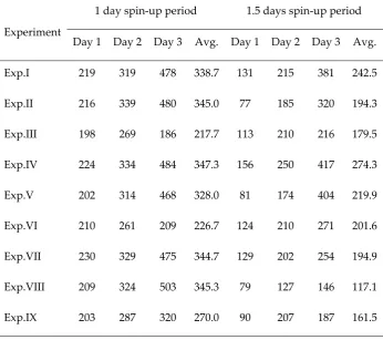
Table 4. As in Table 3, but derived by NCEP-FNL IC/BCs.
282
Experiment
1 day spin-up period 1.5 days spin-up period
Day 1 Day 2 Day 3 Avg. Day 1 Day 2 Day 3 Avg.
Exp.I 219 319 478 338.7 131 215 381 242.5
Exp.II 216 339 480 345.0 77 185 320 194.3
Exp.III 198 269 186 217.7 113 210 216 179.5
Exp.IV 224 334 484 347.3 156 250 417 274.3
Exp.V 202 314 468 328.0 81 174 404 219.9
Exp.VI 210 261 209 226.7 124 210 271 201.6
Exp.VII 230 329 475 344.7 129 202 254 194.9
Exp.VIII 209 324 503 345.3 79 127 146 117.1
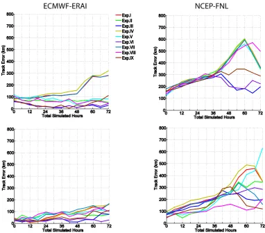
A summary of TC tracking error under the differences of IBCs and spin-up period conditions is
283
shown in Figure 7. The GD scheme showed a small tracking error increasing after 48 hours of
284
simulation testing comparing with the JTWC best track data and other Cu-schemes. Therefore, the
285
KF and BMJ schemes were eliminated in the selection of Cu-physical parameterization schemes for
286
TC Durian simulation in the SCS. The KF and BMJ schemes created quite large tracking errors
287
during the time of strong influence in the upwelling area with high SST variability by updating SST
288
during the WRF-ATM model simulations in the SCOV (i.e. between 4 and 5 December 2006). The TC
289
intensity was discussed in terms of MSLP and Vmax with above stated set of combinations. General
290
consideration and comparative study for model simulation (up to 72 hour forecast) and its
291
approximation were presented in the middle and bottom panels of Figures 5 and 6 (i.e. Vmax and
292
lowest center of MSLP). The MSLP at the lowest center of JTWC observed data was around 976 hPa
293
at 1800 UTC 4 December 2006 in the SCOV. It clearly showed that the GD combinations
294
(Experiments III, VI and IX) were close to the observed central pressure (972.3, 974.4, and 982.4 hPa),
295
especially one day spin-up time for the TC simulation by using the ECMWF-ERAI IBCs.
296
297
Figure 7. Track error (km) of model experiments and a comparison of ECMWF-ERAI (left column) and
298
NCEP-FNL IBCs (right column); same (top row) and different (bottom row) spin-up periods by using the
299
WRF-ATM model simulations of nine experiments, associated with JTWC best-track data from 0000 UTC 2
300
December to 0000 UTC 5 December 2006.
301
However, the WSM6-GD combination (Experiment VI) simulated the intensity of 6 hour
302
forecast from 1800 UTC 4 December to 0000 UTC 5 December 2006 in the SCOV. It provided better
303
result than that of other combinations for convective parameterization and analysis. In the
304
accompanying analysis of TC simulation testing, the combination of WSM5-KF, WSM6-KF,
305
WSM6-BMJ and THOM-KF could not simulate the intensity of MSLP, while the WSM5-BMJ and
306
THOM-BMJ combinations simulated better TC intensity than that of previous combination schemes.
307
UTC 2 December 2006 and the corresponding observed track data are presented in the middle panel
309
of Figures 5 and 6 (i.e. different spin-up period considerations). The Vmax during the simulation
310
period obtained from the JTWC best track data was around 90 knots at 1800 UTC 2 December to 1200
311
UTC 3 December 2006. The THOM-GD combination scheme (Experiment IX) simulated the
312
maximum wind of 87.7 knots, whereas the WSM5-GD and WSM6-GD combination schemes
313
(Experiments III and VI) simulated Vmax of 76.5 and 78.0 knots, respectively, at 0600 UTC 3 December
314
2006 for 1 day spin-up time by using the ECMWF-ERAI IBCs.
315
The combinations of WSM5-KF, WSM5-BMJ, WSM6-KF, WSM6-BMJ, THOM-KF and
316
THOM-BMJ schemes, the Vmax was underestimated by the WRF-ATM model simulation, especially
317
comparing with the THOM-GD combination scheme. However, the intensity simulated by these
318
three combinations of GD scheme, WSM5-KF, WSM6-GD, and THOM-GD, was relatively similar to
319
the trend of Vmax for 6 hour forecast from 1800 UTC 4 December to 0000 UTC 5 December 2006 in the
320
SCOV. For the KF and BMJ Cu-convective schemes, the TC simulations presented the lack of exact
321
location, time and intensity by using both IBCs. The KF is indicated as a complex mass flux scheme
322
with closure assumption depending upon the Convective Available Potential Energy (CAPE)
323
removal for an entraining parcel. The BMJ is classified as a convective adjustment scheme for
324
temperature and moisture profiles. The GD is modified for a one-dimensional mass flux scheme in a
325
single updraft–downdraft couplet. In this study, the KF and BMJ Cu-schemes presented a lack of
326
low level convergence and a decrease of convective activity in development of cyclonic system was
327
also shown. The result indicated that the GD combination schemes and their convection with the
328
entire MP-schemes showed better skill for the TC potential track and its intensity at the strong
329
influence of the upwelling area with high SST variability in the SCOV compared with other schemes
330
and observed track data.
331
3.2. Simulations with Different Spin-up Period, Initial and Boundary conditions
332
Based on the model results of physical parameterization schemes and their combinations, the
333
model simulation was applied for the TC Durian case study with different spin-up time and IBCs of
334
both global models (ECMWF-ERAI and NCEP-FNL) in order to evaluate the model accuracy and
335
performance testing in terms of location tracking and intensity. Figures 5–7 demonstrate the TC
336
Durian track simulations with different spin-up period and IBCs. All the TC tracking simulations
337
were demonstrated with 72 hour predictions by using the WRF-ATM model consideration from
338
0000 UTC 2 December to 0000 UTC 5 December 2006 at every 6-hour time interval. It is interesting to
339
note that all pink boxes along the JTWC best-track data are indicated for the time, location and
340
intensity point of the daily consideration under the difference of spin-up period conditions (Figures
341
5–7).
342
For the initial study of spin-up processes for tuning up the TC simulation, the WRF-ATM model
343
15-km grid has “cold started” using both IBCs that are nested to the WRF-ATM 4-km grid. Based on
344
the cold start, a typical spin-up period of approximately 4-6 hours is conducted before the
345
WRF-ATM develops stable, coherent wind and pressure systems. Thus, it could be stated that the
346
forecast guidance is most useful for time periods beyond 6-12 hours. Several researches with 0000
347
UTC convection-allowing WRF-ATM model simulations revealed that the model could provide very
348
effective guidance for afternoon and evening TC activity [26,27]. A similar spin-up period is,
349
however, explicit in the 1200 UTC WRF-ATM. The useful guidance, thus, might not be provided
350
until the afternoon time period (1800 UTC) at the earliest. In this study, the model testing has been
351
designed for several spin-up experiments in a range of 12-36 hours (e.g. 0.5, 1 and 1.5 days), while
352
the model selection showed only the model convergence which produced the best simulation
353
comparing with the JTWC potential track, Vmax and MSLP. For the model divergence, the weakness
354
simulation results as a spin-up period for 1.5 days by using the ECMWF-ERAI IBCs and 0.5 days by
355
using the NCEP-FNL IBCs have not been presented in this study.
356
For both IBCs, the WRF-ATM model has been used for a period of 1 day starting at 0000 UTC 1
357
December 2006. The second experiment focused on the model generalization capability of speeding
358
up for the model running was also presented in this section. The WRF-ATM model using the
ECMWF-ERAI IBCs started at 1200 UTC 1 December 2006, while the simulation using the
360
NCEP-FNLIBCs began at 1200 UTC 30 November 2006. However, the model experiments using the
361
ECMWF-ERAI IBCs performed well are determining the TC center for 0.5 days and 1 day spin-up
362
periods. Overall, the TC tracks simulated by the ECMWF-ERAI IBCs with both spin-up periods
363
showed better results than those of the NCEP-FNL IBCs comparing with the JTWC observed track.
364
In particular, prior to a 48-hour forecast, the TC tracking error of the ECMWF-ERAI IBCs remained
365
lower than 100 km, while that of the NCEP-FNL IBCs tended to substantially increase with respect to
366
time for all experiments as shown in Figure 7 associated with Tables 3 and 4. Overall, a one-day
367
period of spin-up time taken by the NCEP-FNL IBCs drive to perform the TC tracking location
368
showed northward bias and the TC moved quickly towards land at 1200 UTC 3 December 2006 as
369
compared with the JTWC observed track. The GD combinations of all physical parameterizations in
370
Experiments III, VI, and IX were consistent with the observed track in terms of location tracking for
371
the upwelling area in the SCOV as presented in Figures 5–7 and Table 4. The vector displacement
372
error of TC tracking location under the difference of IBCs and spin-up times is concluded in Figure 7
373
associated with Tables 3 and 4.The best choice of TC tracking simulation was summarized as the
374
WSM5-GD combination in Experiment III. Mean displacement errors at the 24, 48 and 72 hour
375
forecasts (average daily forecast errors) were 39, 15 and 22 km, respectively, with an entire
376
simulation period of 25.3 km.
377
The model results of the GD Cu-scheme with three MP schemes have also been consistent
378
throughout the WRF-ATM model experiments with the mean displacement error within 50 km over
379
the 3-day simulation period. It is worth noting that the location tracking errors of model results
380
comparing with the JTWC observed track were different in all the model simulations and varied
381
from 15 to 503 km with an average range from 25.3 to 347.3 km. However, the model could bring
382
these average location errors to the minimum of 25.3 km in a 72 hour forecast at strong influence of
383
upwelling area with high SST variability. The model result, therefore, suggests that the best choice of
384
the model performance testing could minimize the location tracking error and also bring it down to
385
25.3 km average location error by using the ECMWF-ERAI IBC as shown in Table 3.
386
In all nine simulations for both IBCs with different spin-up periods, except the entire model
387
simulations of the NCEP-FNL IBCs, the model simulated upwelling areas ahead of the actual site in
388
the SCOV. The location tracking error at the high SST variability significantly decreased from 503 to
389
22 km on Day 3 (average daily rate) through the simulations from 0000 UTC 2 December to 0000
390
UTC 5 December 2006. For the analysis of different spin-up periods, the model results clearly
391
illustrated good agreement with the JTWC observed track in terms of location for 0.5 and 1.5-day
392
spin-up periods of both IBCs especially at the first of average daily vector displacement error (Day
393
1). The TC location tracking error depicted small average displacement errors to 21 km by using the
394
WSM5-GD and WSM6-GD combinations for the ECMWF-ERAI IBCs as shown in Experiments III
395
and VI of the top panel in Figure 7 and summarized in Table 3. It also presented the lowest location
396
error of 46 and 29 km at the last average simulation time (Day 3) in the SCOV as shown in Table 3
397
and the top left panel in Figures 5 and 7. For the TC simulations of the NCEP-FNL IBCs, the model
398
results presented an overestimation of vector displacement error in terms of location tracking. Their
399
simulation time was also longer than the previous simulation for 12-hour simulation testing.
400
However, the present results indicate that the model shows the moderate location tracking
401
improvement for a 1.5-day spin-up period. The TC intensity study and analysis of Vmax and MSLP
402
under the Wind-Pressure Relationships (WPRs) have been determined in the next section.
403
3.3 Analysis of the Relationship between Wind Speed and Pressure
404
For nine physical parameterizations and their combinations under the difference of global IBCs
405
and spin-up period conditions, the model results and analysis of simulated intensity such as the
406
Vmax and MSLP have been generally compared to depict the relationship between the TC
407
simulations along with JTWC observed track data for a 72-hour time frame of model consideration
408
(Figures 5 and 6). In this section, the intensity analysis under the WPRs is used to understand the
simulated Vmax and MSLP results. It was accurately presented in the model comparison of each
410
experiment (Experiments I–IX) with five operational agency equations (Opa.I–V) in term of Vmax
411
and MSLP for the quadratic curved lines as shown in Figures 8 and 9.
412
413
414
Figure 8. Wind-Pressure Relationships (WPRs) by WRF-ARW model experiments (marker points) by
415
ECMWF-ERAI (left column) and NCEP-FNL IBCs (right column); same (top row) and different (bottom row)
416
spin-up periods, JTWC best-track data (pink squares) with five operational agency curves (dashed line), TC
417
model simulations illustrated by scatter plots for 15 minutes and JTWC curve line recomputed by using the
418
Atkinson and Holliday [23] equation (JTWC-Opa.III as a black cross-solid line).
420
Figure 9. As in Figure 8, but for model results and specify selected by Opa.III and JTWC-Opa.III curve lines for
421
model consideration. The daily intervals of track locations are shown in the pink squares.
422
These figures show that the JTWC best-track data (pink squares) with its black cross-solid line
423
(JTWC-Opa.III) was the general quadratic function which was computed by the Atkinson and
424
Holliday equation (Opa.III). In this study, the intensity simulation of model experiments using the
425
ECMWF-ERAI IBCs with the mapping quantitative data points for 1 day spin-up period was only
426
one of four package sets for the highest consistency of model simulation with five operational
427
agencies (Opa.I–V). In particular, the simulated Vmax and MSLP showed that the model could
428
capture the TC intensity at peak strength and also under the frame of reference of operational
429
agency curved lines and the JTWC observed data as shown in Figures 8 and 9.
430
The model results of the ECMWF-ERAI IBCs suggest that sampling of TC peak strength could
431
be represented by a full range of intensities which gave sufficient sample size for a 1 day spin-up
432
period.The significant interactivity discrepancies were found in the stronger intensity range. The
433
particular intensified value of the TC simulations tended to present a larger MSLP than that of the
434
observed trend (JTWC-Opa.III). However, the model results of the ECMWF-ERAI IBCs with a 1 day
435
spin-up period represented the best choice of all package sets for decision making under the
436
spin-up period considerations of TC intensity study and analysis. The simulations also show the
437
scatter points closed with the operational agency curved lines which can be directly seen through
438
the data distribution under different spin-up period and IBCs conditions. In addition, the bounded
439
set of scatter simulated results located between five operational agency line curves were the most
440
clearly illustrated guide to the scientific scene of the model simulation and comparison as shown in
441
the top left panel of Figures 8 and 9. The results could be understandably presented by the relation
442
of model scattering points, JTWC intensity points (pink squares) and JTWC-Opa.III observed line
443
original Opa.III curved line by Atkinson and Holliday equations (dashed line). Furthermore, the
445
larger sequences of gaps between the model experiments and observation were noticed at the
446
scaled main and time frame considerations as shown in the middle and bottom right panels of
447
Figures 5 and 6. The model results also apparently presented an underestimation of Vmax and
448
overestimation of MSLPunder the considerations of model spin-up period, validation and analysis.
449
Explicitly, the simulation results of NCEP-FNL IBCs presented the scatter points spreading out and
450
over the operational agency curved line (Opa.I) by the Dvorak [21] equation as shown in the right
451
panel of Figure 8.
452
For the ECMWF-ERAI IBCs with 12 hour-spin up period, the results presented low model
453
accuracy as those initialized by the NCEP-FNL IC/BCs. Although the three package sets using
454
different IBCs and spin-up period considerations which simulated the TC intensity showed some
455
deficiencies, they provided some confidence in the ability of model to reproduce located tracking
456
errors for the model study on the spin-up period considerations. Nevertheless, the fact that model
457
results could be presented without the reinforcement of other operational agencies and were
458
understandably illustrated by the simulated Vmax and MSLP as clearly presented in the top left
459
panel of Figure 9. The results under different IBCs and spin-up period conditions by the WPRs
460
showed that the upper and lower bounds of model simulations were scattered inside the frame of
461
reference for five operational agencies with their curved lines which could predict the cyclone
462
intensity in terms of Vmax and MSLP (Figure 8).
463
In summary, the model results have been illustrated in the quadratic curved diagrams by the
464
WPRs (Figure 10). It showed the analysis diagram of MSLP versus Vmax with the issues of model
465
intensity for the sensitivity results by the smooth ascending and descending trends of both
466
parameters. The curved lines applied by the ECMWF-ERAI IBCs represented the excellent results. It
467
also provided an excellent map with the closed curve of density distribution by comparing with the
468
NCEP-FNL IBCs. In addition, Vmax and MSLP presented the quantitative dependent variables with
469
the line segment that connected several points on the graph (Figure 9). It expresses a quadratic
470
curve which is interpreted visually relative to both variables under the WPRs as shown in the
471
precise Opa.III equation.
473
Figure 10. Quadratic curve lines illustrate model experiments (solid lines) by ECMWF-ERAI (left column) and
474
NCEP-FNL IBCs (right column); same (top row) and different (bottom row) spin-up periods, associated with
475
JTWC best-track data (pink squares), JTWC-Opa.III curve line and its smooth descending trend (black
476
cross-solid line) with various five operational agency equations (dashed lines).
477
Interestingly, the influence of model spin-up period consideration and analysis has a relatively
478
large impact on the reduction of the scatter which described for decreasing the statistical variance
479
explained by the quadratic curved diagram as shown in Figure 10. The model results of the
480
ECMWF-ERAI IBCs with 1 day spin-up period gave the closed curves with the JTWC intensity
481
observed points, JTWC-Opa.III observed curved line and the original Atkinson and Holliday
482
equation (Opa.III). In contrast, the model experiments of the NCEP-FNL IBCs presented the
483
underestimation of simulated results comparing to the JTWC best-track data and the results
484
simulated by the ECMWF-ERAI IBCs. In addition, the model results under the WPRs were finally
485
concluded for the statistical verification and analysis in TC intensity (Tables 5 and 6).
486
Table 5. Statistical error analysis of Vmax (in knots) given by MSLP (in hPa) for Vmax computation with different
487
spin-up periods.
488
Experiment ERAI-1 day ERAI-0.5 days FNL-1 day FNL-1.5 days
Bias RMSE STDE Bias RMSE STDE Bias RMSE STDE Bias RMSE STDE
Exp.I -1.45 2.64 2.21 -2.16 3.67 2.98 -2.44 4.09 3.27 -3.33 5.53 4.41
Exp.II -0.72 1.85 1.70 -5.40 8.54 6.62 -5.02 8.15 6.42 -7.40 11.57 8.89
Exp.III -0.69 1.83 1.70 -2.05 3.55 2.90 -1.91 3.23 2.61 -1.78 3.14 2.59
Exp.IV -1.49 2.62 2.15 -1.94 3.32 2.69 -2.08 3.51 2.83 -2.68 4.49 3.61
Exp.V -1.48 2.72 2.28 -3.44 5.58 4.39 -6.10 9.69 7.53 -4.46 7.20 5.65
Exp.VII -1.25 2.34 1.98 -3.15 5.11 4.02 -2.11 3.52 2.82 -4.04 6.64 5.26 Exp.VIII -0.74 1.85 1.70 -4.26 6.90 5.42 -3.17 5.15 4.06 -7.36 11.56 8.92
Exp.IX -0.74 1.88 1.73 -2.87 4.76 3.79 -1.22 2.28 1.92 -1.94 3.38 2.77
489
Table 6. As in Table 5, but for MSLP (in hPa) given by Vmax (in knots).
490
Experiment ERAI-1 day ERAI-0.5 days FNL-1 day FNL-1.5 days
Bias RMSE STDE Bias RMSE STDE Bias RMSE STDE Bias RMSE STDE
Exp.I -0.83 1.83 1.63 -1.18 2.28 1.95 -1.17 2.28 1.95 -1.17 2.23 1.90
Exp.II -0.56 1.67 1.57 -1.48 2.68 2.23 -1.42 2.61 2.18 -1.72 3.01 2.47
Exp.III -0.43 1.69 1.63 -0.94 2.05 1.82 -1.38 2.58 2.18 -1.04 2.12 1.84 Exp.IV -0.82 1.85 1.66 -1.06 2.11 1.82 -0.99 2.04 1.78 -1.01 1.99 1.72
Exp.V -0.96 2.01 1.77 -1.57 2.85 2.38 -1.90 3.27 2.66 -1.16 2.23 1.91
Exp.VI -0.39 1.66 1.61 -0.64 1.80 1.68 -1.09 2.24 1.95 -0.94 1.99 1.76
Exp.VII -0.82 1.82 1.62 -1.21 2.31 1.97 -0.95 1.95 1.70 -1.17 2.25 1.91 Exp.VIII -0.36 1.64 1.60 -1.32 2.46 2.07 -1.59 2.81 2.32 -1.76 3.06 2.51 Exp.IX -0.35 1.64 1.60 -0.91 2.01 1.79 -0.66 1.83 1.71 -0.87 1.92 1.71
491
The comparison of intensity simulation of curved line results and observed track reanalyzed
492
by the Opa.III equation was rather small for the model validation. The simulated MSLP tended to
493
be significantly lower than observed intensity with similar Vmax for the analysis of Bias. The
494
simulation agreed well with the method and analysis results reported by Islam et al. [6]. It was
495
found weakening/steady and intensifying storms had different WPRs and the intensity trend of a
496
given storm was suggested by the shapes of those curves. This was also a key factorto determine
497
the WPRs. Using different IBCs and spin-up periods, the differences found by Atkinson and
498
Holliday [23] were confirmed for the simulation and analysis in this work. The research findings of
499
this study showed that the intensity of storm simulations for a 1 day spin-up period of the
500
ECMWF-ERAI IBCs had a tendency to capture lower pressures and stronger winds comparing with
501
those of other spin-up periods, especially for the model experiments using the NCEP-FNL IBCs
502
with its spin-up periods. The simulated results had a weakening/steady and intensifying for storm
503
considerations. These simulations were further examined in the next discussion of intensity
504
summary and analysis by using the WPRs.
505
For the WPRsin terms of the statistical analysis indexes (e.g. Bias, RMSE and STDE), the model
506
simulations and observational curved lines by the Opa.III smooth descending trend of Vmax and
507
MSLP under the WPRs were used to mathematically express a trend of modeling and observational
508
data as summarized in Tables 5 and 6 and corresponded in Figure 10. In this study, the
509
WRF-ATM model experiments indicate that the simulated intensity with different IBCs and spin-up
510
periods by the Opa.III smooth descending trend of Vmax and MSLP under the WPRs could also be
511
directly influenced by the physical parameterizations and selection through the model experiments.
512
The simulated results with statistical analysis using the WSM5 and WSM6 MP-schemes were found
513
to have lower Vmax and MSLP than those with the THOM scheme during 3-daysimulated time (72
514
hour forecast) of the super typhoon Durian case study. The results demonstrated that the WSM5
and WSM6 MP-schemes with GD Cu-scheme provided lower accuracy and performance testing
516
than those of the THOM MP-scheme with GD Cu-scheme throughout the entire simulations.
517
In this study, the summary results show the WPRs curved fitting with Vmax given by MSLP in
518
nine physical combinations for different IBCs and spin-up period experiments. The WPRs have
519
been used to derive the Vmax approximations by the statistical analysis indexes as demonstrated in
520
Table 5. The best choice of physical parameterization by the WSM5 and GD Cu-schemes which
521
simulated by using the NCEP-FNL IBCs with 1.5 day spin-up period (Exp.III) provided relatively
522
low Bias of -1.78 knots (RMSE = 3.14, STDE = 2.59). As expected, the model experiment simulated by
523
using the ECMWF-ERAI IBCs with a 1 day spin-up period (Exp.III) yielded the lowest statistical
524
errors in comparison with a Bias of -0.69 knots (RMSE = 1.83, STDE = 1.70). In contrary to derive the
525
MSLP given by Vmax for the TC reanalysis, Table 6 presents the statistical error of MSLP. The
526
Experiment IX combination with a 1 day spin-up period led the lowest Bias of -0.66 knots (RMSE =
527
1.83, STDE = 1.71) by the NCEP-FNL IBCs and Bias of -0.35 knots (RMSE = 1.64, STDE = 1.60) by the
528
ECMWF-ERAI IBCs, among all investigated combinations.
529
In addition, the cyclone made landfall on 5 May 0000 UTC, produced widespread strong winds
530
and pressure drops over the SCOV region. This study discusses the 24-hour location tracking and
531
its intensity such as Vmax and MSLP from JTWC observed data and model simulated location and
532
intensity for three corresponding days valid at 0000 UTC of 3, 4 and 5 December 2006. In the final
533
analysis, Figures 11–14 represent the 72 hour wind and sea level pressure fields valid at 0000 UTC 5
534
December 2006 derived from simulated location tracking (pink line), JTWC observed track data
535
(black line) and the final 72 hour simulation of model consideration (pink square) corresponding to
536
the above period of three experiments (Experiments III, VI and IX) from the best choice of model
537
physical parameterizations of full integration system from 0000 UTC 2 to 0000 UTC 5 December
538
2006.
540
Figure 11. Summary of model experiments in term of wind fields (m/s) at the 10-meter height level selected by
541
model accuracy and performance testing, associated with JTWC best track data (black-solid line). Experiments
542
III, VI and IX with their simulated TC tracks (pink cross-solid lines) by using ECMWF-ERAI (top), NCEP-FNL
543
(middle), and different IBCs (bottom) at 0000UTC 5 December 2006 for 1 day spin-up period.
545
Figure 12. As in Figure 11, but for surface level pressure fields (hPa).
547
Figure 13. As in Figure 12, but for wind fields (m/s) and its different model spin-up periods of ECMWF-ERAI
548
0.5 days (top), NCEP-FNL 1.5 days (middle) and different IBCs (bottom).
550
Figure 14. As in Figure 13, but for surface level pressure fields (hPa) and its different model spin-up periods.
551
552
In general, the model was able to capture the wind and sea level pressure fields well at the TC
553
center position and can be compared with the JTWC analysis for 3 days. It is noteworthy that the
554
simulations captured the TC center position well at the strong influence of upwelling area with
555
high SST especially in the SCOV by using the ECMWF-ERAI IBCs with both spin-up periods, while
556
it was underestimated by using the NCEP-FNL IBCs. The 24-hour wind and sea level pressure
557
fields at the TC center position valid at 0000 UTC 3 December 2006 from JTWC analysis provided
558
northward bias above the TC simulations by using both IBCs with a 1 day spin-up period in the
559
SCS (Figures 11 and 12). The simulations for Day 1 forecasting from 0000 UTC 2 to 0000 UTC 3
560
December (average daily rate) capture the TC center position reasonably well by using the
561
ECMWF-ERAI IBCs with 0.5-day spin-up period (Figures 13 and 14). The JTWC intensity for
562
24-hour analysis valid at 0000 UTC 3 December 2006 illustrated the wind damage associated with
563
increasing TC intensity from 75 (Category 1) to 90 knots (Category 2) over the SCS. In addition, the
564
TC simulation slightly underestimated the Vmax for the three physical combinations by both IBCs
565
and different spin-up experiments over the SCS. However, the simulations of 0000 UTC 5 December
of a 72-hour forecast shows that the model could capture the TC center position well over the
567
upwelling zone in the SCS, especially for the Experiment III using the ECMWF-ERAI IBCs with a 1
568
day spin-up period. The wind and sea level pressure fields show high intensity over the SCS, while
569
the TC center position moved toward from the SCS to the GoT. All model experiments, excluding
570
the NCEP-FNL IBCs used (middle panel of Figures 11 and 12) with a 1 day spin-up period of 0000
571
UTC 5 December of 72-hour forecast agreed reasonably well with the JTWC observed tracking, and
572
successfully predicted the TC location tracking and its intensity of Vmax and MSLP. However, the
573
Experiment III predicts less MSLP, while the Experiment IX shows the best MSLP results by using
574
the ECMWF-ERAI IBCs with a 1 day spin-up period as the schemes mentioned above. A
575
comparison of the JTWC observed analysis and model prediction indicates that the model was
576
successfully able to simulate the TC location tracking, Vmax and MSLP in terms of model sensitivity
577
analysis and performance testing as well as intensity. Differences of IBCs, spin-up period and
578
physical combination schemes could provide better understanding of global model uses through
579
WRF-ATM simulation and sensitivity of model physics describing the physical processes in natural
580
phenomena.
581
4. Conclusions
582
In this study, the best combination of nine sensitivity experiments on various physical
583
parameterization schemes under the difference of IBCs and spin-up periods for 36 experimental case
584
studies has been performed with the WRF-ATM modeling system to predict super typhoon Durian
585
over the SCS. The model results of the sensitivity experiments revealed that the TC intensity was
586
controlled by cumulus convection and TC track prediction was affected by the microphysics
587
parameterization schemes.
588
Although the model has underestimated the intensity with all sensitivity experiments, the
589
combination of WSM5 MP-scheme with the GD Cu-scheme by using the ECMWF-ERAI IBCs with a
590
1 day spin-up period (Experiment III) showed better prediction with MSLP error of 1.69 hPa and
591
Vmax error of 1.83 knots under the WPRs. The WSM6 and THOM MP-schemes with the GD
592
Cu-scheme for Experiment VI and Experiment IX gave the MSLP error of 1.66 and 1.64 hPa,
593
respectively, whereas the Vmax error of both experiments was about 1.88 knots - more deviated from
594
the observed data. The dynamical processes of TC location tracking and its intensity were also well
595
captured by the WSM5–GD schemes (Experiment III) in terms of TC center position and Vmax.
596
Furthermore, the combination of physical parameterization schemes, the TC simulations were
597
initialized with different IBCs and spin-up period experiments for a 0.5, 1 and 1.5-day model
598
considerations from 0000 UTC 2 to 0000 UTC 5 December 2006. The simulations with various initial
599
conditions indicate that the model is capable of prediction of cyclone intensity in terms of MSLP and
600
Vmax during the peak period in the SCS and the strong influence of upwelling area with high SST
601
variability in the SCOV. The displacement error of the TC simulation was well predicted by using
602
Experiment III with an average vector displacement error of 25.3 km (approximately 25 km) in 72
603
hours. The present results demonstrate that the GD scheme and its combinations could successfully
604
predict intensity in terms of MSLP and Vmax.
605
Overall, the WRF model shows excellent skill for the TC Durian prediction in terms of location
606
tracking and intensity, suggesting that the model has the potential to be used for operational
607
forecasting systems especially applied for a coupled model with SST updating. In addition, the
608
model could produce the potential and intensities of TC simulation reasonably well over the SCS.
609
The results of this study would benefit other TC simulations and forecasting under similar
610
conditions to Durian in 2006. In this study, the TC simulation is still a challenging to research and
611
extensive in scope; it is available for model improvement such as precise vortex relocation, model
612
initialization and data assimilation as well as other available observations for fully coupled data
613
assimilation with the TC system developments. The model resolution, various physical