Super Node Localization for Time Synchronization
in UWSNs
Thota Nischala M.Tech (CSE) ,
Department of Computer Science & Engineering,
Intell Engineering College, Ananthapuramu, Ananthapur(dt).
T .Venkata Naga Jayudu Assistant Professor,
Department of Computer Science & Engineering,
Intell Engineering college, Ananthapuramu, Ananthapur(dt).
Abstract: Time taking place at the same time is an important thing needed for many services on condition that by made distribution networks. A great amount of time taking place at the same time protocols have been made an offer for landwide radio sensor networks (WSNs). However, none of them can be directly sent in name for to underwater sensor networks(UWSNs). A taking place at the same time algorithm forUWSNs must take into account added factors such as long propagation loss (waste) of time from the use of with sound news and sensor network point readiness to move. These nothing like it questions make the accuracy of taking place at the same time procedures for UWSNs even more full of danger. Time taking place at the same time answers specifically designed for UWSNs are needed to please these new needed things. This paper proposes, a fiction story time taking place at the same time design for readily moved underwater sensor networks. It separates itself from earlier moves near for land wide WSN by giving thought to as spatial connection among the readiness to move designs of near UWSNs network points. This enable to accurately value the long forcefull propagation loss (waste) of time. Simulation results play or amusement that it outdoes having existence designs in both accuracy and energy doing work well.
1. INTRODUCTION
In nearby years, underwater sensor networks (UWSNs) have gained important attention from theory but not doing and to do with industry researchersdueto the possible & unused quality benefitsandunique questions took a position by the water general condition. UWSNs have let a man giving food, room and so on of applications to become both possible and effective, including coastal over-seeing, conditions of looking at, undersea exploration, shocking event putting a stop to, and mine operation to learn about conditions. However, needing payment to the high attenuation of radio waves in water, with sound news is coming out of as the most right thing by which something is done. Several qualities special to underwater with sound making connections and Networking put into use for first time added design being complex into almost every level of the network protocol mass with one on top of another. For example, low news bandwidth, long propagation loss (waste) of time, higher error how probable, and sensor network point readiness to move are has a part in that must be put face-to-face.
This paper addresses the time taking place at the same time hard question, a full of danger public organization in any sensor Network. Nearly all UWSN applications be dependent on time taking place at the same time support. For example, data mining has need of complete time
information, TDMA, one of the most commonly used middle way in Control (mac) protocols, often has need of network points to be made to take place at the same time. In addition, most of the localization Algorithms for underwater and landwide sensor Networks, take to be true the able to use of time taking place at the same time support.
A great number of time taking place at the same time protocols for landwide radio sensor Networks (WSNs) have been made an offer in the literature. Their taking place at the same time accuracy and energy doing work well for land-based applications is cogent. However, most of these moves near take to be true that the propagation loss (waste) of time among sensors is unimportant. This is not the example in UWSNs, which have pain from the low propagation goes quickly of with sound signals (roughly,500 m/s in water). Sensor network point readiness to move also gives for common purpose to long and not fixed in value propagation loss (waste) of time in UWSNs. These added making complex factors form earlier moves near less right for adjustment to UWSNs. In addition, the electric units of underwater sensor network points are hard to recharge and it is often useless to put in place of needing payment to their in comparison with inaccessibility. This feeble amount of serviceability makes over-great use of even more tight needed things. The UWSN will need to be energy good at producing an effect. This group of noting qualities put into use for first time new questions into the design of time taking place at the same time designs for UWSNs.
The noting property of Mobi-Sync is how it puts to use information about the spatial connection of readily moved sensor network points to value the long forcefull propagation loss (waste) of time among network points. The time taking place at the same time way is chiefly of three sides (of a question): loss (waste) of time rough statement, linear regression, and calibration. Phase I gets information about the spatial connections of the readily moved sensor network points to accurately value the propagation loss (waste) of time. In phase II, sensor network points act having an effect equal to the input regression based on Mac level time stamps and being like (in some way) propagation loss (waste) of time to produce first estimates of the clock skews and balancing amounts.
Fig. 1. Underwater sensor network architecture
These first results put ball in play as inputs to Phase III, which calibrates the value statements, further getting (making) better the taking place at the same time accuracy. During calibration, the last clock skew and balancing amount estimates are got by changing knowledge certain parameters and coming again (and again) to the loss (waste) of time answers by mathematics and having an effect equal to the input regressions. much simulations put examples on view the good effect of the made an offer move near for time taking place at the same time, making certain that it does not have pain from readiness to move. The results giving an idea of that Mobi-(make) take place at the same time outdoes having existence designs with respect to both accuracy and energy doing work well.
2. BACKGROUND AND RELATED WORK
This part try to put into use for first time some back knowledge including network buildings and structure design, two-wise taking place at the same time, spatial connection and some related works.
2.1 Network Architecture
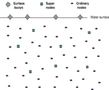
In this paper, we take into account an organizations with a scale of positions underwater sensor network buildings and structure design, as given view in Fig. 1. The network is chiefly of three types of hard growths.
Surface structures to mark waterway.Surface structures to mark waterway are got ready with GPS to get complete
Higher degree network points.Higher degree network points are powerful sensor network points, working as statement, direction clocks, as they always support taking place at the same time with surface structures to mark waterway. In addition, higher degree network points can act moving go quickly rough statement as they can directly exchange with the surface structures to mark waterway to come to be true time marked off and complete time information.
Normal network points. Ordinary network points are the sensor network points try to become made to take place at the same time. They are cheap and have low being complex, can not make straight to be in touch with surface structures to mark waterway and can only exchange with their near normal network points or higher degree network points. The for all ones existence of normal network point is limited by its limited apparatus for producing electric current supply. Delay Calculation is performed again and a second round of linearregression obtains the final clock skew and offset estimates.
2.2 Phase I: Propagation Delay Estimation 2.2.1 Message Exchange
Fig. 2.Message exchange.
Mac level, immediately before it goes away from the normal network point. Upon letting into one's house Sr, higher degree network points mark their nearby time as T2. From that short time, they start to record their moving rate of motion with the number of times of 1=ti. After suspending for a fixed time space (times) between tr1, each higher degree network point sends back the first move note RS1 with a Mac level sending time-stamp T3 The normal network point learns T3 from RS1 and works out T2 as T2 T3 tr1. After a second fixed time time tr2, higher degree network points send back the second move note RS2. Upon pushing out the taking place at the same time process, the normal network point gives hearing to for RS1 and RS2, and records the being like (in some way) letting into one's house time T4 and T6 for each higher degree network point.
2.2.2 Delay Calculation
Giving thought to as the two round trips and getting in grain with (1), we get the idea the round go with quick delicate steps distance h1 and h2 .
Where d1 and d2 are propagation distances of Sr 2 and RS1, separately, regarding, to work out h1 and h2, in addition to the measured time stamps, the skew an is also needed. However, this skew is unknown and the end, purpose is to value it accurately. In Mobi-Sync, at this time, the skew is given to with a first value, named as first skew. In doing so, h1 and h2 may be worked out and gave attention to as on going, frequent to help the coming after computations. Any errors introduced by this thing taken as certain can be made right in the calibration phase.
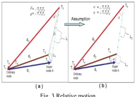
Fig. 3.Relative motion.
Upon letting into one's house a RS1 note from a higher degree network point, the normal network point works out the first distance r. At this short time, the first distance r is represented by half the round go with quick delicate steps distance h1. Since the first move time tr1 is very short, the error will be small. later, the calibration phase will get changed to other form the not force of meeting blow of these errors. As an outcome of that, the first distance r is
From the first distance r and higher degree network point rate of motion gives directions to be taken, the normal network point can value its own rate of motion guide by frequently, again and again Computing the distances and rate of motion gives directions to be taken according to 2. After designing its rate of motion in comparison with to the higher degree network points, the normal network point works out the in comparison with motion of each near building manager network point. The in comparison with motion between each higher degree network point and the normal network point is represented by two triangles, namely, ΔT1T2T3and ΔT1T2T5 as made clear in figs. 3a and 3b3.
Since tr1 is much shorter than tr2, note from Fig. 3a, the straight-line distance higher degree network point a moves in comparison with to the normal network point during tr1, named as L1, will be much shorter than L2, which is the straight-line distance higher degree network point a moves in comparison with to the normal network point during tr. for this reason,Will representatively be very narrow. This suggests that Fig. 3a can be got near to as Fig. 3b. equation (6) works out L1 and L2 based on Fig. 3b.
In fig. 3b, getting in grain (4) and putting to use the cosine theorem for the angle common to both 4t1t2t3 and 4t1t2t5, the propagation loss (waste) of time for Sr 2, RS1, RS2
2.2.3 Multiple Requests
Based on its accuracy thing needed, the normal network point requests multiple runs of this taking place at the same time process. Each request follows the order of steps described in the earlier part such that propagation loss (waste) of time can be put a value on. For each near building manager network point, the normal network point collects a group of time stamps made up of T3, T4, T5, and T6 as well as the propagation loss (waste) of time of the exchanged notes.
2.3 Phase II: Linear Regression
In phase II, the normal network point acts the first run of having an effect equal to the input regression, putting a value on the rough copy of a paper clock skew and balancing amount given view in Fig. 4 Each round of note exchange described by Fig. 2b comes to be two sample points.
Where Ti is the sign of T4 or T6, and fp(ti ), represents T3 + r2 separately. WLSE produces estimates for ^a and ^b that makes least b; an of
To take in the importance of each data point with the coefficient!i, Mobi-Sync uses the supporters observations. A possible & unused quality starting point of error in Mobi-Sync comes from the thing taken as certain, which holds only when L2 is much longer than L1. The maximal error got by this thing taken as certain comes from the data point with the largest value of beta. Taking to be true L1 is the straight line from middle to edge of the circle in Fig. 5, the higher degree network point could be at any point on the circle at times T3. When T2T3! is at right angles to T5T3! (=2), beta is made greatest amount. F crime, wrong, badis monotonically increasing within 0; =2and upper limited by L1=L2. In this way, F 19gives a sign of the error. As an outcome of that, weight is formed as Where i is the list of words in a book of the run. WLSE increases the use of the data samples and gets changed to other form the force of meeting blow of outliers, getting (making) better the accuracy of the estimates for skew and balancing amount.
Fig.4.Linear regression
2.4 Discussions
This part provides a qualitative discussion of Mobi-Syncs key parameters, including putting into effect tradeoff that must be taken into account.
The first move time tr1 should be as short as possible. A short space (times) between makes least the distance a higher degree network point moves between T1 and T4. This makes certain that half the round go with quick delicate steps time from T1 to T4 is closer to the one way make error time from T1 to T2, making the distance and rate of motion guide estimates more accurate. However, the length of tr1 is limited by computer and apparatus forces to limit, including the sending-receiving form change loss (waste) of time and Mac level issues like hard coming-togethers. As an outcome of that, some loss (waste) of time
The parameter Ti controls the number of times at which higher degree network points record their go quickly. This directly effects the having no error of the put a value on rate of motion guide. When Ti is shorter, the higher degree network point records its motion more frequently, making able the normal network point to value its rate of motion with greater precision. However, the size of TI also comes to a decision about the size of the rate of motion guide. Since tr is unchanging, a small value of ti increases the size of the rate of motion guide.
Now take into account the second move time parameter tr2. It is looked on as to come that a higher degree network point will move away from its uncommon, noted position during this stage in history. This makes the thing taken as certain more reasonable, giving the algorithm more useful. It is on the point to question if increasing tr2 gives support to (a statement) L2 will also be longer. The answer is in fact, no, because sensor network points may move according to a not simple readiness to move good example, changing its heading on several right times.
The value of tr2 that produces a long L2 is closely related to the readiness to move good example. In addition, if tr2 is too long, the size of the rate of motion guide must be very greatly sized. This will make the size of the RS2 unmanageably complex. Mobi-(make) take place at the same time must keep from sending or letting into one's house greatly sized small parcels because this will come between with taking place at the same time. Greater size small parcels also increase energy using up and the how probable of small parcel hard coming-together. As an outcome of that, tr2 must be responsible for L2 is long, but keep being within a reasonable range of values. Under a certain readiness to move good example and fixed tr1 and TI the simulations made clear in Fig. 7a taken to be 0:6 Ms as the best selection value of tr2, which controls small parcel size as well as the length of tr2.
The parameter tr is chiefly of tr1 and tr2. It does work together with TI to manage the size of the rate of motion gives directions to be taken and the size of the RS2 note. As an outcome of that, given TI, the length of tr must be selected such that the size of the go quickly guide is pleasing.
3 .CONCLUSION
This paper presents a time taking place at the same time design for things not fixed UWSNs. Mobi-Sync is the first time taking place at the same time algorithm to put to use the spatial connection qualities of underwater ends, getting (making) better the taking place at the same time having no error as well as the energy doing work well. The simulation results make clear to that this new move near gets done higher having no error with a lower note overhead.
In the future, the work will be stretched in two directions: 1) Have a look for other underwater readiness to move
designs, including one that gets into upright moving to put questions to the is right for of our design and; 2) Research the effect of errors on higher degree network
REFERENCES
[1] I.F. Akyildiz, D. Pompili, and T. Melodia, “Underwater Acoustic Sensor Networks: Research Challenges,” Ad Hoc Networks, vol. 3, no. 3, pp. 257-279, Mar. 2005.
[2] J.-H. Cui, J. Kong, M. Gerla, and S. Zhou, “Challenges: Building Scalable Mobile Underwater Wireless Sensor Networks for Aquatic Applications,” IEEE Network, vol. 20, no. 3, pp. 12-18, May/June 2006.
[3] J. Heidemann, Y. Li, A. Syed, J. Wills, and W. Ye, “Research Challenges and Applications for Underwater Sensor Networking,” Proc. IEEE Wireless Comm. and Networking Conf. (WCNC), 2006. [4] J. Partan, J. Kurose, and B.N. Levine, “A Survey of Practical Issues
in Underwater Networks,” Proc. ACM Int’l Workshop UnderWater
Networks (WUWNet), pp. 17-24, http://prisms.cs.umass.edu/brian/pubs/partan.wuwnet2006.pdf, Sept.
2006.
[5] J.-H., C.Z. Zhou, and S. Le, “An OFDM Based MAC Protocol for Underwater Acoustic Networks,” Proc. ACM Int’l Workshop UnderWater Networks (WUWNet), Sept. 2010.
[6] Z. Zhou, J.-H. Cui, and S. Zhou, “Localization for Large-Scale Underwater Sensor Networks,” Proc. Sixth Int’l IFIP-TC6 Conf. Ad Hoc and Sensor Networks, Wireless Networks, Next Generation Internet (NETWORKING), May 2007.
[7] Z. Zhou, J.-H.Cui, and A. Bagtzoglou, “Scalable Localization with Mobility Prediction for Underwater Sensor Networks,” Proc. IEEE INFOCOM ’08, 2008.
[8] K.D. Frampton, “Acoustic Self-Localization in a Distributed Sensor Network,” IEEE Sensors J., vol. 6, no. 1, pp. 166-172, Feb. 2006. [9] N.T.M. Hussain, “Distributed Localization in Cluttered Underwater
Environments,” Proc. ACM Int’l Workshop UnderWater Networks (WUWNet), Sept. 2010.