CENTRE FOR
ADV
ANCED
SP
A
TIAL
ANAL
YSIS
W
orking Paper Series
Paper 61
AGENT-BASED
PEDESTRIAN
MODELLING
Centre for Advanced Spatial Analysis University College London
1-19 Torrington Place Gower Street
London WC1E 6BT
[t] +44 (0) 20 7679 1782 [f] +44 (0) 20 7813 2843 [e] [email protected] [w] www.casa.ucl.ac.uk
http//www.casa.ucl.ac.uk/working_papers/paper61.pdf
Date: January 2003
ISSN: 1467-1298
© Copyright CASA, UCL
Agent-Based Pedestrian Modelling
Michael Batty
Centre for Advanced Spatial Analysis, University College London, 1-19 Torrington Place, London WC1E 6BT, UK
1
To be published in P. A. Longley and M. Batty (Editors) Advanced Spatial Analysis, ESRI Press, Redlands, CA, in the press.
Agent-Based Pedestrian Modelling
Michael Batty
Professor of Spatial Analysis, Director CASA, University College London, 1-19 Torrington Place, London, WC1E 6BT, United Kingdom
webhttp://www.casa.ucl.ac.uk/people/Mike.htm email[email protected])
Abstract
2
1 Spatial dynamics at the fine scale: agents and infrastructure
As we approach scales where geometry in the form of streets, buildings, and land parcels becomes significant, the focus of inquiry in urban modelling changes from one where location is dominant to situations where the local dynamics of movement are much more significant. This is easily illustrated in retailing. Firms fix their general location according to geodemographic patterns of demand and the availability and capacity of infrastructure, but their precise locations are determined according to the volumes of trade generated by their competitors. In turn these depend not only on footfall in shopping streets but also on the ways in which goods are positioned relative to movement patterns of shoppers within the stores themselves. These ideas are manifest in the rules of thumb used by retail planners in organising the layout of shopping malls where stores position themselves according to the way their products relate to each other and to the position of the anchor stores that heavily influence the overall character of any given retail development.
Until quite recently these kinds of problem were seen as lying outside the remit of urban modelling and GIS. However, advances in computation– in terms of the acquisition of digital data using sensors, improved storage and processing of disaggregate data, and advances in object-oriented programming which make it possible to represent and simulate large numbers of generic objects or agents – have enabled us to make substantial progress, some of which we will report in this Chapter. Conceptual developments too in dealing with dynamic systems at aggregate (see Batty and Shiode, this volume) and disaggregate levels (see Torrens, this volume) combined with ideas from complexity theory enabling us to link seemingly uncoordinated actions at the local level with the emergence of more global structures (see Longley et al, this volume) are providing the intellectual framework. Central to this is the idea of agents in which behaviour is simulated as a trade-off between selfish and unselfish actions, between individual and cooperative decision-making. The classic case can be seen in local movement where the desire to reach some goal often leads to turbulence in crowd situations while the desire to see what others are doing leads to flocking. Both can end either in congestion and panic or in smooth movement if local actions develop at speeds which allow synchronisation.
3
available to planners and engineers, notwithstanding the need for strategies to enable their integration. They also pose important challenges to GIS for they involve geometry in a way that has not been central to spatial analysis and they invoke a concern for dynamics that has long been an Achilles’ Heel of geography and GIS. The models that we will sketch out here all deal with pedestrian movement in streets, buildings and related complexes, and introduce ideas about variability and heterogeneity in urban systems which are largely defined away in the more aggregative applications which characterise mainstream GIS applications. The way in which randomness, geometry, and economic and social preferences combine and collide will in fact be our starting point and this introduces a very different mix of modelling styles than any developed in this field hitherto. The nexus of this emerging field arises from the synthesis between randomness and geometry in physics, related to ideas concerning economic rationality and social preference.
We will begin with ideas about hypothetical walks – random walks, adding geometry and economy as we go, thus constructing a generic model of local movement. We illustrate the approach in the rest of the Chapter by applying it to three very different situations: very fine scale street situations dominated entirely by geometry and the collective phenomena of crowding and panic; more economically structured movements characteristic of shopping behaviour in centres and malls; and managed situations such as festivals and street parades where control is essential to public safety.
2 Random walks, geometry, and locational preference
4
in the physical world there are particles; in the natural world, plants and animals; and in our own domain – the human world – there are ourselves but also the agencies and institutions we create to produce collective responses. The way in which randomness, geometry, and intention combine is different in each of these domains. Modern physics, for example, is largely a product of randomness with the constraining effect of geometry, whereas modern economics is the product of randomness with distinct preferences which imply sentient behaviour. In human spatial systems at the level of the agent, behaviour is more complex in that it is clearly some product of randomness, geometry, economic intentions, and social preference.
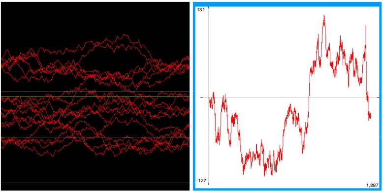
Figure 1: A one dimensional random walk
(A) the walk wraps around from left to right every 200 time periods; and (B) the walk over its 1387 time periods
5
process where the lag in value of the stock is one time period (one-order) and is often called a Markov process. In Figure 1, we show an example of the behaviour of this process where we have simply simulated variation from the starting point of v(0)=0 for some 1400 time
periods. Every 200 time periods the value wraps around in Figure 2A but we show the entire series in Figure 2B where it is clear that if you examine a small part of the series and then scale this up – aggregate it over time – the series is self-similar or fractal, a well known characteristic of this kind of constrained randomness.
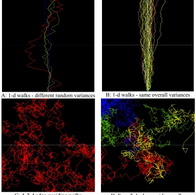
To think of this kind of walk as a walk in human space, we only need to think of Figure 1 as simulating how a human agent walks forward along the y=0 line. Time thus becomes the forward direction and the randomness is a sideways deviation. If the apparent magnitude of the random variation in this Figure suggests that our human agent is intoxicated, do remember that the amplitude of the random variation would appear much less if the y axis were marked in larger increments, and that there is always some random deviation to help us to steady ourselves when walking. Thus in Figure 2A, we show four different walks all from the same starting position where the blue walk has the least variation, the yellow a little more with the green more still: the red line might be associated with someone who has had too much to drink! In Figure 2B, we keep the variance the same but start a series of walkers from the same point and track their paths. Because change is random, some vary quite a lot but there is a clear tendency for the walks to bunch together with the deviations from the straight line following a Normal Distribution.
It is easy to write our generic model now for this kind of walk. Using x and y for the coordinates of each point on the walks in Figures 2A and 2B, then
+ = + + = + 1 ) ( ) 1 ( ) ( ) 1 ( t y t y t x t
x εx
(1)
where is it very clear that our walk is highly constrained in the y direction. It is now very simple to turn this walk into a 2-dimensional random walk. In a sense it already is but if we fix change in the y direction randomly just as we have done in the x direction, that is we set
y
t y t
6
randomly but at least does not go outside the space – that is the walker avoids the edges – and in Figure 2D, we show the course of four walkers doing the same. If we let these walkers continue in this way, then at the scale of resolution at which we are viewing the space, then all the pixels in the space will soon be visited and the 1-d tracks will come to fill the 2-d space. This is another example of randomness being fractal in that here is an example of a space filling curve – a line of one dimension filling a space of dimension 2 – an object with a Euclidean dimension of 1 but a fractal dimension of 2.
A: 1-d walks - different random variances B: 1-d walks - same overall variances
C: A 2-d edge avoiding walks D: Four 2-d edge avoiding walks
Figure 2: Multiple one and two-dimensional random walks in the same 2-d space
7
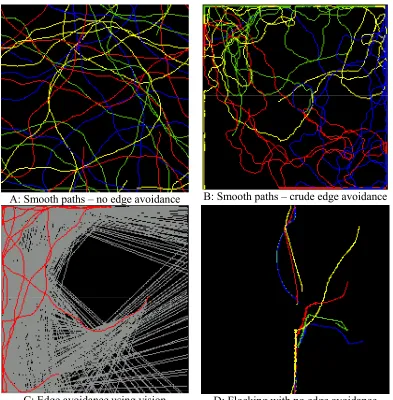
geometry of the environment begins to constrain and give structure to such random walks but first let us note that as soon as we begin to make assumptions about how the walker moves, we, unwittingly perhaps, introduce behaviour. The walks in Figure 2 twist too violently in terms of direction for these to be characteristic of the way human beings respond and if we constrain such twists, producing the sort of gentler walks that we show in Figure 3A, then we simulate greater realism. It is clear that there are two very different ways in which the walk can be constrained to avoid crossing the edge of the space. The rather blunt way is that whenever a walker bumps against the edge, the walker then shifts away from the edge, while the more intelligent way is that the walker sees the edge long before it is reached and takes evasive action. The first way which is shown in Figure 3B, simply constrains the walker from crossing the edge but is dominated by movement along the edge. The intelligent way requires a lot more computation. From any position the walker must look ahead and determine how far from the edge it is, then alter its heading in such a way that as it gets nearer to the edge, it veers away from it, thus retaining its smooth behaviour. We show such a strategy in Figure 3C where the grey lines are lines of sight computed from every point where the walker is located. Note how the track, shown in red, can be altered according to how far the walker is from the edge. This is akin to introducing vision into our system but this is expensive in terms of computer time for it means that before a walker moves, it must have information about how far every possible move is from every possible obstacle.
8
way groups of people coalesce and disperse in situations of crowding. We show the tracks of such behaviour for four agents who flock together and wrap from the top to the bottom of the screen in Figure 3D.
A: Smooth paths – no edge avoidance B: Smooth paths – crude edge avoidance
C: Edge avoidance using vision D: Flocking with no edge avoidance
Figure 3: Smooth walks (A), edge avoiding (B), with vision (C) and with clustering-flocking (D)
9
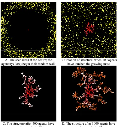
terminate once they reach any fixed point: for example, plant a fixed point at the centre of a space and then launch a series of walkers at a far distance from this point, letting them walk randomly in the space. As soon as one of the walkers ‘touches’ this point, it creates another adjacent point and then moves far away from the growing structure. If this process continues what happens is that the structure grows in a treelike manner away from the initial point, creating a growing structure such as that shown in Figure 4 for three time periods.
A: The seed (red) at the centre; the
agents(yellow) begin their random walk B: Creation of structure: when 100 agents have touched the growing mass
C: The structure after 400 agents have
come into contact with it D: The structure after 1000 agents have come into contact with it
10
Basically this is a good model of how a street system might grow in a town over a long time period. People migrate into the space and wander around until they come into contact with each other; once they do so, they decide to settle and if the walkers are launched one at a time, then eventually the growing structure tends to fill the space available. The criterion for settlement is immediate adjacency to the existing structure and, as the walkers are more likely to come into contact with its edges, growth mainly takes place on the edge of the structure’s growing tentacles. This is called diffusion limited aggregation (DLA). At the most local level in terms of movement within streets, there is some sense in which such patterns do reflect the location of shops on radial roads emanating from a town centre, thus reflecting location which is the product of movement (migration) over a much longer time periods than those used in the models produced here. Once again such structures are fractals, this DLA model being at the core of much recent work on thinking of city morphologies as fractals (Batty and Longley 1997).
3 Movement at the very fine scale: a generic model
We now need to stand back and derive a generic model for local movement from the ideas we have already introduced. All the elements of this have been stated, at least implicitly, and there are at least four features that direct movement. First geometric obstacles need to be negotiated. Second agents repel each other when congestion and crowding builds up, while third, agents are attracted to each, these second and third features being the elements used in flocking. The fourth element though in one sense the most important, relates to the desired direction in which the walker wishes to travel. In our random walks, we assumed that this was either straight ahead or completely random but in real situations, we must generate such directions as the product of preferences and intentions. A useful formulation of these ideas has been developed over several years by Helbing and his group (Helbing et al, 2001). Helbing (1991) refers to his generic model of pedestrian movement as a social force model in which each of these four features is associated with a force that pushes the walker in a particular direction. In general we might think of movement to a new location as being formed from
ε + + + + + = attraction social repulsion social repulsion geometric position desired position old position new
11
where each of these components is some function that is ‘added’ into the algorithm that is used to compute movement. Desired position is a behavioural variable which relates to locational preferences while geometric repulsion is the summation of forces which stop a walker from bumping into some obstacle. Vision is important in its computation. Social repulsion and attraction are summations of all the interaction effects with other agents that are within the neighbourhoods or fields where such effects are relevant to movement.
There are several ways in which this formulation can be made operational. At very fine scales where panic and crowding are the main behaviours as in evacuation and emergency situations, the model can be formulated traditionally in terms of the physics of motion where velocity and acceleration play a central role (Helbing et al 2000). Where speed is not important then the coordinates of position can form the essence of computation (or headings if this be the preferred form: see Batty et al, 1998) while in situations where location is relative, then pixel location relative to local neighbourhoods can be used as in traditional spatial interaction modelling (Batty et al 2003). In fact in computation associated with such models, there is no simple equation structure, because motion must be computed through a sequence of decision rules that incrementally update position.
12
In Figure 7, we show a situation where there are two types of pedestrian: those forming a parade which moves around the corner of a street intersection (agents in white) with pedestrians watching (agents in red). The model enables us to assess the build up in pressure between the two types of walker and to set a threshold which if breached, leads to one crowd mixing with the other. This is achieved in Figure 7B where the red agents build up pressure in trying to see the parade (social attraction) but then try to diffuse (social repulsion) with serious consequences in that the only way this can happen is the for the crowd to panic and break through the parade into freer space. This is the kind of disaster scenario that such models can be used to predict.
A: Walkers move from left to right B: The attraction surface
C: Agents reaching the desired location D: Agents cluster at the desired location
13
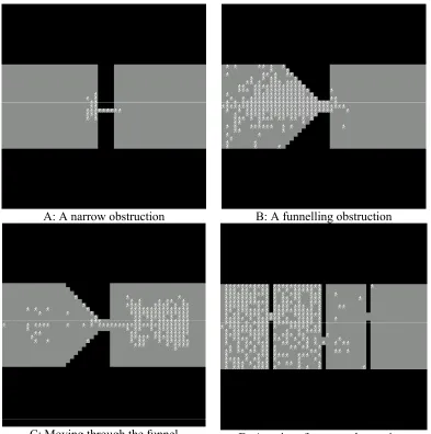
A: A narrow obstruction B: A funnelling obstruction
C: Moving through the funnel D: A series of narrow obstructions
Figure 6: How obstructions delay movement, and compromise safety
14
4 Individual and collective behaviour: pedestrians in buildings, malls and centres
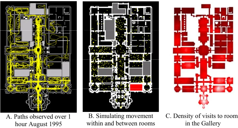
Our first application is to a complex building – the Tate Britain art gallery in London, UK – which currently houses the Gallery’s classical collection, although when our study was undertaken, the Gallery also housed the modern collection now in the Tate Modern. The Space Syntax group at UCL (http://www.bartlett.ucl.ac.uk/research/space/overview.htm) specialises in recording pedestrian movement in buildings and they carried out a survey of movement through the rooms of the Gallery over a one week period in August 1995. The building provides an excellent test bed for simulating local movement as there is only one entrance but many rooms and corridors which contain very different paintings and sculptures – thus providing a clearly differentiated set of destinations for art lovers and the more causal visitor alike. In many respects, the kind of movements associated with the Gallery are not too dissimilar from those associated with browsing when shopping and thus the applications provided a rather good problem on which to fine tune the model.
Figure 8A shows the pattern of movements recorded by the Space Syntax group over one hour in August 1995 using a technique of person following which the group had perfected in many other studies. It is clear from these patterns that the Gallery has a greater number of visitors on the left hand side of its central axis where the classical and British collection was housed in contrast to the rather sparser number of person movements associated with the right hand side where the modern collection was kept. It is unclear whether this is reflects the preferences of the visitors or the more convoluted room structure associated with the right hand side – or indeed whether it reflects various perceptual clues associated with lightness in the Gallery once they enter. The book shop – in red in Figure 8B – is also a major focus for movement having a somewhat different purpose from the rest of the Gallery.
15
vision into the structure by pre-processing. The pre-processing stage involved computing the visual (isovist) fields associated with each pixel point describing the Gallery (Batty 2001). Social repulsion related directly to density limits on crowding and if breached resulted in dispersion within a local neighbourhood; social attraction was based on a flocking like algorithm which enabled visitors to follow others if it appeared that flows to particular rooms were increasing. Fluctuations based on the random walk behaviour that we used in the 1-D walks in Figures 2A and 2B were also incorporated to reflect variations in walking behaviour within a large and heterogeneous population. We also experimented with some versions of the model where the number attracted to rooms changed the attraction surface associated with the rooms, starting with a version where all the rooms were equally attractive and seeing how a hierarchy of attraction evolved through movement. A typical output of the model is shown in Figure 8B where the yellow dots relate to the 550 or so walkers observed in the Gallery during the one hour period when the observations were made.
A. Paths observed over 1 hour August 1995
B. Simulating movement
within and between rooms C. Density of visits to rooms in the Gallery
Figure 8: Observation and simulation of visitors within the Tate Britain Gallery
16
of application. We show the pattern of room densities which was computed over many runs of the model where the walkers moved around the Gallery for many time periods, in Figure 8C. Here is it clear that from a starting position where all the rooms had equal attraction, the asymmetry of movement actually observed in the Gallery was simulated by the model in its steady state. We can say little more than this although the implication is that it is the configuration of the Gallery rather than what is on its walls and in its rooms that conditions how people move within it. We can also use the model rather effectively to close and open certain rooms. The bookshop for example is a case in point (see the red room in Figure 8B) and if this is closed then the pattern on the right hand side of the Gallery changes substantially.
17
physical and locational structure of activities in the centre becomes associated with the preference of the shopper.
This framework has been elaborated in CASA using the well known SWARM modelling system designed to simulated artificial life forms. Haklay et al (2001) developed such a model where preferences and geometry were combined in a much more sophisticated way than in the model shown here. In fact in the model whose typical output in shown in Figure 9, shoppers only visit the centre for a fixed period of time with an increasing number returning to their rail and bus stations and car parks while others enter the centre. In this way we are able to build the routine dynamics – the ebb and flow of shoppers during the shopping day – into the model and thus begin to asses critical densities at particular points in time. In this way, we can begin to get a handle on locational attraction not only in space but also in time and this leads us full circle to ideas about the 24 hour city and the way retailers are beginning to compete in time.
Figure 9: Simulating pedestrian shopping trips from car parks in Wolverhampton Town Centre (within the ring road – mapped extent 1km square)
5 Highly managed spatial events: street parades and carnivals
18
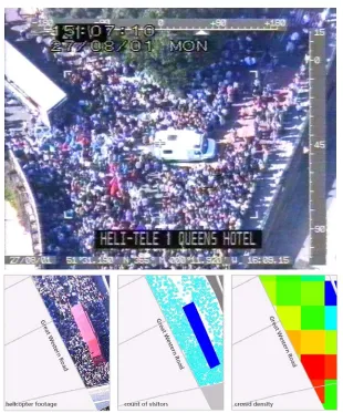
reflecting various preferences for places and goods, movements associated with street festivals and parades are in a sense simpler, more focused locationally but in another sense, more complex in that walkers and visitors respond less predictably to stimuli that together comprise the event. We have built a model of an annual street festival in west central London that is known as the Notting Hill Carnival. The Carnival has grown from a small West Indian street celebration first held in 1964 to a two-day international event attracting 710 000 visitors in 2001. It consists of a continuous parade along a circular route of nearly 5 kms in which 90 floats and 60 support vehicles move from noon until dusk each day. Within the 3 km2 parade area, there are 40 static sound systems, and 250 street stalls selling food. The peak crowds occur on the second day between 4pm and 5pm when in 2001, there were some 260 000 Carnival visitors in the area. There were 500 accidents, 100 requiring hospital treatment with 30 percent related to wounding, and 430 crimes committed over the two days with 130 arrests. Some 3500 police and stewards were required each day to manage the event.
The safety problems posed by the event are considerable. There are many routing conflicts because of cross movements between the parade and sound systems while access to the Carnival area from public transport is uneven with four roads into the area taking over 50% of the traffic. A vehicle exclusion zone rings the area, and thus all visitors walk to the Carnival. Crowd densities are high, overall at about 0.25 persons per m2; a density of 0.47 ppm2 line the Carnival route while there are 0.83 ppm2 inside the route where the sounds systems are located. We have good data for crowd densities from our own cordon survey, data on entry/exit volumes at London Underground (subway) stations, and 1022 images of the parade taken by police helicopters in the early afternoon of the second day. We show some of these images in Figure 10 from which we have extracted detailed crowd density statistics throughout the area. What we do not have are good data on the paths taken by the visitors from their points of entry into the Carnival area to the various attractions that comprise the event: however, most visitors enter using one of 38 entry points, with half the volume associated with 5 entry points related to subway stations, and this simplifies the application.
19
different attractions which make up the entire event with respect to the points where visitors enter and then simulates how these agents walk to the event from these entry locations. In events such as these, we are never in a position to observe the flow of pedestrians in an unobstructed manner because the events are always highly controlled. We have thus designed our model in three stages. First, we build accessibility surfaces from information inferred about how walkers reach their entry points (origins) relative to their ultimate destinations at the Carnival. Second, we use these surfaces to direct how walkers reach the event from their entry points and then assess the crowding that occurs. Finally we introduce controls to reduce crowding, changing the street geometry and volume of walkers entering the event, operating this process iteratively until an acceptable solution is reached. These three stages loosely correspond to exploration, simulation, and optimisation.
Figure 10: Crowd density at the Notting Hill Carnival
20
In the first exploratory stage, we begin with walkers located at their ultimate destinations in the Carnival area. Walkers move randomly from location to location (which we refer to as cells), avoiding inaccessible cells which are obstacles such as buildings and barriers. The probability of moving from one cell to another is computed according to the accessibility of that cell, which in turn is based on the number of walkers having already visited the cell. At the beginning of this process, all cells have the same probability but eventually a walker will discover an entry point to the Carnival – an origin – and when it does, the walker switches from exploratory to discovery mode and returns to the destination with knowledge of the discovery. As the destination is known in that the walker has come from this, it lays a trail back to its source akin to the way ants drop pheromone once they have discovered a food source and head back to their nest (Camazine et al 2001). When the walker enters the neighbourhood of its destination, it switches back to exploration mode and the search begins over again.
21
The exploratory stage finishes when the walkers converge on an efficient and unchanging set of paths between the entry points (origins) and the attractions (destinations) which define the
A C E
B D F
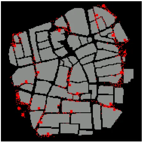
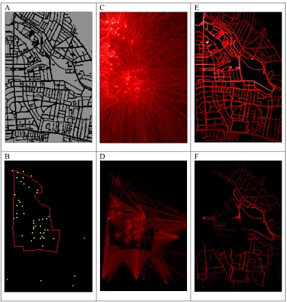
Figure 11: Exploration of the street system and discovery of entry points (tube stations) in Notting Hill
(A) the street geometry; (B) the parade route (red), sound systems (yellow), and subway stations (blue); (C) accessibility from parade and sound systems without streets; (D) shortest routes to subway stations without streets; (E) accessibility with streets; and (F) shortest routes with streets. Relative intensities (of accessibility)
are shown on a red scale (light = high; dark = low). Scale: horizontal width of each map is 1.7 kms.
22
from stage 1 to condition the probabilities of movement. There are two effects that complicate this of which the first is flocking (social attraction). This directs movement as an average of all the movement in the immediate neighbourhood of a walker (Reynolds 1987; Vicsek et al 1995). But the second effect indicates that a move only takes place if the density of walkers in any cell is less than some threshold based on the accepted standard of 2 persons/m2. If this is exceeded, the walker evaluates the next best direction and if no movement is possible, remains stationary until the algorithm frees up space on subsequent iterations. These rules are ordered to ensure reasonable walking behaviour. This second stage is terminated when the change in the density of walkers in each cell converges to within some threshold where it is assumed a steady state has emerged.
We can assess how good the model is at predicting the observed distribution of crowds using a battery of statistical tests based on densities and paths and if the model survives, we move to the third stage which is more informal. Note that so far we have not introduced controls on where people are able to move for we begin with no street closures or barriers used in crowd control. In a sense, the Carnival is never without any control so our third stage is to introduce such controls, one by one, to ensure that we produce a safe simulation as well as showing what might be achieved under certain strategies. We do this by examining statistics from the second stage, and gradually making changes to reduce the population at risk by introducing barriers, capacitating entry points, and closing streets. As the repercussions of this are not immediately obvious, we make these changes one by one, re-running the model until an acceptable solution emerges. In estimation, this stage may also be used to assess the efficacy of existing controls. It is not possible to develop a formal optimisation procedure as so many additional factors such as resources for policing etc. cannot be embodied in the model. Nevertheless we consider this interactive method of introducing control the best approach so far for assessing alternative routes.
23
significant points of crowding. We predict around 72% of the variance of the observed densities for 120 locations where good data are available. At the third stage, we rerun the
A C E
B D F
Figure 12: The full modelling sequence and identification of vulnerable locations
(A) the 2001 parade route (red and green) with proposed 2002 route in red, sound systems (yellow), and entry points (blue); (B) composite accessibility surface from stage 1; (C) traffic density from stage 2; (D) areas closed by the police used in stage 3; (E) location of walkers in the stage 3 steady state; and (F) vulnerability of locations
predicted from stage 3, on a red scale (light = high; dark = low).
24
crowding have been removed. This suggests that even in estimating the model, it can be used in a diagnostic manner to identify vulnerable locations as we show in Figures 12E and 12F.
We can now use the model to test alternative routes as we did in the full project (ISP 2002). After considerable political debate, an interim change in route was agreed for Carnival 2002 where the northernmost section of the parade (shown in Figure 12A in green) was removed. Running the model leads to slightly reduced average crowding but other problems associated with starting and finishing the parade not included in this model, emerge. The process of changing the Carnival route is still under review with better data being collected each year. Many of the problems of using this model interactively with those who manage the event are being improved. As we gain more experience of this approach, we are better able to adapt this kind of model to different policy making situations.
6 The future: fine scale dynamics and GIS
In this Chapter we have shown how a focus on finer scales of granularity than GIS is typically concerned with, throws up problems of representation and dynamics which are hard to embody within traditional GIS. Clearly the models we have been dealing with are part of an enhanced geographic information science but a focus on the fine, localised scales where human action and motion is to the fore, reveals that traditional GIS is largely concerned with systems which are represented in terms of their inanimate characteristics. Insofar as human activities are represented in GIS, these are in static, aggregative terms. Moreover the kinds of events that this Chapter has been concerned with are much shorter lived than those that are traditionally a part of our science. This is partly because we are only just beginning to get a handle on fine scale events of short duration but it is also because such events now seem more important than ever they were previously as is witnessed in our concern for developing an appropriate science to deal with safety, crime, and leisure.
25
phenomena but once the concern shifts to dynamics and to fine spatial scales, then fusing traditional GIS with these kinds of models and analysis becomes an even greater challenge. The kind of fusion that has been attempted quite successfully by Evans and Steadman (this volume) for land use-transport models is not possible with the models of this Chapter, because the processes and scales involved are too different from the way traditional software in information systems has evolved. Nevertheless, what we have shown here is that the fine scale of granularity and its dynamics are rich in detail and that the visualisation that is involved in making sense of these events is consistent with the traditions of GIS. We have raised many new issues in this Chapter which we see as some of those to which GIS needs to respond to as it becomes increasingly adopted and adapted in urban policy-making where physical design and social action are integral to relevant human action.
7 References
Batty M 2001 Exploring isovist fields: space and shape in architectural and urban morphology. Environment and Planning B, 28: 123 – 50
Batty M, Desyllas J, Duxbury E 2003 Safety in numbers? modelling crowds and designing control for the Notting Hill Carnival. Urban Studies, forthcoming
Batty M, Jiang B, Thurstain-Goodwin M 1998 Local Movement: Agent-Based Models of Pedestrian Flows. Working Paper 4, Centre for Advanced Spatial Analysis, University College, London; available at http://www.casa.ucl.ac.uk/local_movement.doc
Batty M, Longley P 1994 Fractal Cities: A Geometry of Form and Function. Academic Press, San Diego, CA
Batty M, Longley P 1997 The fractal city, Architectural Design, 67 (9-10: Profile 129): 74-83. Bonabeau E, Dorigo M, Theraulaz G 1999 Swarm Intelligence: From Natural to Artificial Systems. Oxford University Press, New York.
Burstedde C, Klauck K, Schadschneider A, Zittarz J 2001 Simulation of pedestrian dynamics using a two-dimensional cellular automaton. Physica A, 295; 507-25.
Camazine S, Deneubourg J-L, Franks N R, Sneyd J, Theraulaz G, Bonabeau E 2001 Self-Organization in Biological Systems. Princeton University Press, Princeton, NJ.
Dijkstra J, Jessurun J, Timmermans H J P 2002 A multi-agent cellular automata model of pedestrian movement. In Pedestrian and Evacuation Dynamics. edited by M. Schreckenberg and S. D. Sharma, Springer-Verlag, Berlin, 173-80.
Haklay M, Thurstain-Goodwin M, O’Sullivan D, Schelhorn T 2001 So go downtown: simulating pedestrian movement in town centers. Environment and Planning B. 28, 343-59. Helbing D 1991 A mathematical model for the behavior of pedestrians. Behavioral Science. 36, 298-310.
Helbing D, Farkas I, Vicsek T 2000 Simulating dynamical features of escape panic. Nature. 407, 487-90.
26
ISP 2002 Carnival Public Safety Project – Assessment of Route Design for the Notting Hill Carnival, Intelligent Space Partnership for the Greater London Authority, London.
Reynolds, C 1987 Flocks, herds, and schools: a distributed behavioral model. Computer Graphics, 21: 25-34.
Still G K 2001 Crowd Dynamics. PhD Thesis, University of Warwick, Warwick, UK; available at http://www.crowddynamics.com/