On the security of oscillator-based random
number generators
Mathieu Baudet1, David Lubicz2,3, Julien Micolod2, and Andr´e Tassiaux1
1 ANSSI, 51 blv de la Tour Maubourg, 75007 Paris
2 C´ELAR, BP 7419, F-35174 Bruz
3 IRMAR, Universit´e de Rennes 1, Campus de Beaulieu, F-35042 Rennes
Abstract. Physical random number generators (a.k.a. TRNGs) appear
to be critical components of many cryptographic systems. Yet, such building blocks are still too seldom provided with a formal assessment of security, in comparison to what is achieved for conventional cryp-tography. In this work, we present a comprehensive statistical study of TRNGs based on the sampling of an oscillator subject to phase noise (a.k.a. phase jitters). This classical layout, typically instantiated with a ring oscillator, provides a simple and attractive way to implement a TRNG on a chip. Our mathematical study allows one to evaluate and control the main security parameters of such a random source, includ-ing its entropy rate and the biases of certain bit patterns, provided that a small number of physical parameters of the oscillator are known. In order to evaluate these parameters in a secure way, we also provide an experimental method for filtering out the global perturbations affecting a chip and possibly visible to an attacker. Finally, from our mathematical model, we deduce specific statistical tests applicable to the bit stream of a TRNG. In particular, in the case of an insecure configuration, we show how to recover the parameters of the underlying oscillator.
Keywords: hardware random number generators, ring oscillators, jitter model, entropy, statistical tests.
1
Introduction
security, following the recommendations of [12]. This explains our focus on a simple design, suitable for a complete and precise modeling.
A source of randomness commonly used in FPGA and ASIC implementations of TRNGs is the instability of signal propagation time across logic gates. This instability is typically accumulated in so-called ring oscillators, consisting in a series of inverters or delay elements connected in a ring. The phase jitter of a ring oscillator is then extracted by means of a sampling unit, for instance a type-D flip-flop triggered by another ring oscillator or by an external clock signal. This simple structure has been widely studied in the literature as a building block for many on-chip TRNGs [8,3,14]. This paper aims to present a comprehensive statistical model of such a basic random unit, and contribute more generally to improving the security analysis of hardware random number generators.
Previous work on provably secure TRNGs based on sampled oscillators in-cludes the work of [11,9,4], who consider mathematical models based on the flipping times Tk of the signal, that is, the times of its rising and falling edges. These models are natural to consider as they correspond to what can be ex-perimentally observed on an oscilloscope. Existing work [9,4,2] report that the durationsXk =Tk+1−Tk between the flipping times appear in many cases to be independent and identically distributed (in shorti.i.d.), as one could expect from the physical intuition of electronic noise. This allows one to compute a safe lower bound of the entropy rate of the TRNG [9]. Yet, we found that such time-oriented models become quickly intractable when one wishes to compute more precise security parameters, such as the maximal bias on a short vector, or the probabilities of outputting certain bit patterns.
Our first contribution is an original approach to address this limitation using a different family of statistical models based on Wiener processes, a classical tool in the study of noisy oscillators [6]. More precisely, we identify the phase of an oscillator to a one-dimensional Brownian motion, and see the outputs of the generator as a (periodic, possibly probabilistic) function of the phase. This new, phase-oriented presentation allows us to achieve exact and approximate formulas for the probabilities of occurrence and for the entropy of arbitrary-length bit vectors, as well as a simple lower bound for the entropy rate. We validate these computations from a physical perspective by arguing, after [6], that the time-oriented and the phase-time-oriented models should be equivalent whenever the jitters of oscillators are small compared to their nominal periods. (This is always verified in practice.) Our formulas take as input a small number of physical parameters that still need to be measured in order to provide a full security assessment.
Our results show that the measure of the statistical parameters of the jitter usu-ally described in the literature [14,4,2] can be inaccurate and, sometimes, largely over-estimated. To solve this issue, we present an experiment able to extract and precisely measure the local Gaussian component of phase jitters, by comparing the signals of two free running oscillators on a same FPGA.
Finally, we apply our formulas to deduce statistical tests directly applicable to the output sequence of a TRNG. Our tests are specifically tailored to detect over-sampled oscillators, and potentially much stronger than the general-purpose tests routinely used [1]. In particular, for a sufficiently large amount of over-sampled bits, we observe that it is feasible to recover the main statistical parameters of a TRNG.
Organization of the paper. In Section 2, we recall the classical, time-oriented models for the sampling of oscillators, then we introduce our new, phase-oriented approach and use it to compute the security parameters of oscillator-based TRNGs. Section 3 presents an experiment designed to extract the Gaussian component of the phase jitter of a ring oscillator. Finally, in Section4, we out-line two special-purpose statistical tests applicable to the outputs of a TRNG in order to assess its statistical properties. Appendices A,Band Ccontain re-lated proofs, additional justifications and an extension to a design made of two oscillators.
2
Statistical models for the sampling of oscillators
Motivated by the example of TRNGs based on ring oscillators, we describe two approaches to model an oscillator subject to phase jitters, and sampled by a time reference (e.g. a quartz clock signal). Whereas the first approach, based on flipping times, is classical [11,9,4], to our knowledge, the second approach, based on a Wiener processes, has never been considered in the field of secure random number generators. We focus on this new approach and derive several formulas to compute the security parameters of a TRNG, notably the biases and the entropy of bit-vectors, and as well as a lower bound of the entropy rate.
For simplicity, in what follows, we keep in line with previous work in the area [11,9,4] and concentrate on symmetric (in particular balanced) oscillators, for which the falling and rising transitions are equally distributed.
2.1 Classical approach (time-oriented)
A common and natural model for jittered oscillators consists in assuming that the half-periods, that is, the durationsXk =Tk+1−Tk between the flipping times
Tk (k ≥ 0) of the signal, are independent and identically distributed random variables. In the sequel, we write mX = E(Xk) for the mean, ands2X = V(Xk) for the variance ofXk.
s(t) is often referred to as analternated renewal process (see for instance [15]). Assuming a start-up time tS and a fixed sampling period ∆t, the successive outputs of the random number generator are finally given bys(tS),s(tS+∆t), . . . ,s(tS+n∆t),. . .
This model has been widely studied in the community of cryptographic ran-dom number generation [11,4], and even generalized [9] to allow for short-term dependencies between the Xk. Notably, Killman and Schindler [9] provide an approximate lower-bound for the source entropy, and present experimental re-sults on a TRNG based on noisy diodes, which appear compatible with the i.i.d. assumption on the Xk.
Although an elegant explicit formula exists for the Laplace transform of P[s(t) = 1] (see [15, p. 334]), to our knowledge there is no general way to com-pute the probabilities of sampling arbitrary-length bit-vectors from alternating renewal processes, let alone if one wishes to abstract away the initial conditions by letting the start-up timetS tend to +∞. Yet, evaluating these probabilities is important to predict residual biases in the outputs of a TRNG, design specific statistical tests, or simply validate the physical model and the amount of Gaus-sian noise at a higher level. For these reasons, we consider another approach that directly models the phase evolution of an oscillator.
2.2 New approach (phase-oriented)
Motivated by typical solutions of equations in the study of noisy oscillators [6], we consider a family of model where the phase ϕ of an oscillator is analogue to a (stationary) one-dimensional Brownian motion. Accordingly, we model the evolution of the phase by a Wiener stochastic process (ϕ(t))t∈Rwith driftµ >0 and volatility σ2 > 0. In other words, for any times t ≥ t0, the phase ϕ(t) conditioned on the values (ϕ(t′))t′≤t0 prior tot0 follows a Gaussian distribution of mean ϕ(t0) +µ(t−t0) and variance σ2(t−t0). Equivalently, in terms of conditional density of probability, we have for allt,t0,x, x0,
d
dxP[ϕ(t)≤x|ϕ(t0) =x0, (ϕ(t
′))
t′<t0 =. . .]
= 1
σp2π(t−t0) exp
−(x−x0−µ(t−t0))2 2σ2(t−t
0)
(1)
where the dots denote any set of values. (Note that bothµandσ2are frequencies here.)
Given a valuex of the phase at a given time t, the output bits(t) is then modeled by a random variable such that the probability of s(t) = 1 is equal to
g1(x), for some fixed 1-periodic functiong1. Letg0= 1−g1be the complementary function. Again, in terms of conditional probability, we have for allt,b,x
P[s(t) =b|ϕ(t) =x, (ϕ(t′), s(t′))t′6=t=. . .] =gb(x). (2) The fact thatg1is 1-periodic is related to the periodicity of the sampled signal, whose average period is thus equal to 1
µ. Another noticeable consequence is that
In the following, we concentrate on the (almost) deterministic sampling pro-cess defined by
g1(x) =
1 ifxmod 1 ∈]12,1[,
0 ifxmod 1 ∈]0,12[,
1
2 ifxmod 1 ∈ {0, 1 2}.
(3)
In other words, for such a choice ofg1, we have thatϕ(t)∈]0,12[ impliess(t) = 0,
ϕ(t) ∈]12,1[ implies s(t) = 1, and ϕ(t) ∈ {0,12} implies that s(t) is a pure random bit. (This last case is negligible and only motivated by Fourier series.) We note that more complex signals, for instance featuring unbalanced and/or noisy sampling, could be modeled as well, simply by adapting the definition ofg1. When no initial precondition is given, we assume thatϕ(0) follows the uni-form distribution on [0,1[, thereby modeling an infinite amount of time spent after the start-up of the oscillator. In particular, this ensures that eachϕ(t0) fol-lows the (same) uniform distribution, and that the source (s(t))t∈Ris stationary, that is, the probabilities of sampling bit vectors are invariant by time-shifting.
2.3 Equivalence formulas between models
For real physical systems, we expect the jitters to be small, that is, σ2 ≪ µ, in terms of Wiener process. Arguably, the sampling of such a Wiener process is equivalent to that of an alternated renewal process where the durations Xk follow an inverse Gaussian distribution (a.k.a. Wald distribution):
pXk(x) =
λ
2πx3
12
exp−λ(x−mX) 2 2m2
Xx
forx >0 (4)
with parameters
mX= 1
2µ and λ= m3X
s2X =
1
4σ2. (5)
Indeed, on the one hand, it is well-known that this distribution corresponds to the first passage time, from ϕ(0) = k
2 to ϕ(x) = k+1
2 , of a Wiener pro-cess with drift µ and volatilityσ2 (see for instance [5, p. 221]). On the other hand, the assumptionσ2≪µallows us to ignore the possibility for the sampled signal to flip in a detectable manner because of the phase going backward: in-deed by another classical result of Wiener processes [5, p. 212], the probability P[∃t≥0, ϕ(t)≤ϕ(0)−α] =e−2ασµ2 will be infinitesimal for meaningfulα >0.
Remark 1. We note that Equation (5) allows one to set the parametersmX and
s2
X in function ofµandσ2, and use other distribution laws forXk. For instance, we may use a Gamma distribution:
pXk(x) =
1
Γ(k)θk x k−1ex
θ (6)
with parametersk= E(Xk)2
V(Xk) =
µ
2σ2 and θ= E(Xk)
k =
In any case, we will have s2X
m2
X
=2σ2
µ ≪1, therefore, we expect that the shape of a given distribution law will have little influence on the behavior of processes. By extension, this suggests that Wiener processes suffice to approximate every physically relevant model based on renewal alternating processes. In the litera-ture of noisy oscillators, we found that Demir et al. [6] do relate phase-oriented processes to time-oriented processes based on Gaussian distributions.
2.4 Controlling bit-vector probabilities, source entropy and biases
Let ∆t > 0 be some fixed sampling period. Using either kind of model, we define thequality factor Q=σ2∆t=s2X∆t
4m3
X of an oscillator-based TRNG as the
phase variance accumulated between two samples, and letν =µ ∆t= ∆t 2mX be frequency ratio between the sampled and the sampling signal.
As mentioned before, in physical random generators based on phase jitter, we expect that Qν = σ2
µ ≪1.
Remark 2. We note that the notion of quality factor is in line with the intuitive definition for a alternating renewal process: the average relative variance accu-mulated during a time ∆t (that is, approximately for ∆t
2 E(Xk) = ν periods) is
given by
ν V(X2k+X2k+1)
E(X2k+X2k+1)2 =ν
2
V(Xk) E(Xk)2
=σ2∆t=Q. (7)
We expect the sampled bits to behave as a perfect random source when the quality factorQis significantly larger than 1. Indeed the accumulated phase jitter between two samples then amounts to more than one period of the oscillator.
In order to make this statement rigorous, we provide several formulas for the probabilities and the entropy of arbitrary-length bit vectors.
Proposition 1. Consider a Wiener process (ϕ(t)) with parameters µ and σ2
and define (s(t))as previously. Letν=µ ∆t andQ=σ2∆t.
1. The probability to sample1at time t≥0conditioned on the phase at time0
verifies
P[s(t) = 1|ϕ(0) =x] = 1 2−
2
πsin(2π(µt+x))e
−2π2
σ2t+O(e−4π2
σ2t). (8)
2. The probability to output a vector b = (b1, . . . , bn) ∈ {0,1}n at sampling
times0, ∆t, . . .(n−1)∆tsatisfies
p(b) =P[s(0) =b1, . . . , s((n−1)∆t) =bn] (9)
= 1 2n +
8 2nπ2
n−1
X
j=1
(−1)bj+bj+1
cos(2πν)e−2π
2
3. The entropy of such an output is
Hn=
X
b∈{0,1}n
−p(b) logp(b) (11)
=n−32(n−1) π4ln(2) cos
2(2πν)e−4π2Q
+O(e−6π2Q). (12)
These expressions result from a careful study of the mathematical model, based on Fourier series and given in appendixA. Our study also provides exact formulas suitable for precise numerical simulations.
Lower bound for entropy. For a stationary process, it is well-known [13] that 1
nHn and Hn −Hn−1 tends (from above) to a same limit H, called the
bit-rate entropy of the source. We emphasize that the approximation of Hn above (Equation (12)) is not provably uniform inn, and thus cannot be used to provide a rigorous lower bound ofH. However, following similar ideas as in [9], it is easy to state a lower bound ofH based on the entropy ofs(∆t) conditioned onϕ(0).
Corollary 1. Let H(s(∆t) | ϕ(0)) = R1
0 H(s(∆t) | ϕ(0) = x)dx denote the
average conditional entropy of s(∆t) with respect toϕ(0), where by definition
H(s(∆t)|ϕ(0) =x) =−plog2(p)−(1−p) log2(1−p) (13)
if p=P[s(∆t) = 1|ϕ(0) =x]. Then we have that
H ≥ H(s(∆t)|ϕ(0)) = 1−π2ln(2)4 e−
4π2Q+O(e−6π2Q). (14)
Remark 3. For a sanity check, note that 4
π2ln(2) ≈0.58> π432ln(2) ≈0.47.
Bounding biases in function of Q and n. We should emphasize that the given approximation forp(b) (Equation (10)) hold whene−2π2Q is small enough for a fixed parameter n=|b|. Preliminary numerical experiments suggest that these approximations might not hold uniformly in n. As a consequence, controlling the biases of the source may require to limit the number of consecutive outputs returned by the random source to not exceed a fixed valuenmax. To help designers assessnmaxin a safe way, we provide exact bounds on the biasesǫ(b) = 2np(b)−1.
Proposition 2. Letϑ(x) =P
k∈Zxk 2
for |x|<1andB =e−2π2Q
. For everyn
and everyb∈ {0,1}n, it holds that|ǫ(b)| ≤ϑ(B)n−1−1. In particular, for every
n such thatn≤nmax=⌊1 + log 1
Q B=e−2π2Q n
max=⌊1 +log2(1ϑ(B))⌋
0.1 1.3·10−1 3 0.2 1.9·10−2 18 0.3 2.6·10−3 130 0.5 5.1·10−5 6701
1 2.6·10−9 129·106 2 7.1·10−18 48·1015
3
Measuring the phase jitter of ring oscillators
In Section 2, we recalled classical models based on flipping times, and showed how to use a new family of models based on Wiener processes to analyze the security of a TRNG. Such security analyses rely on the physical parameters of the generators, that is, the frequency ratioν and a quality factorQ.
In this section, we first report several experiments in order to assess the physical parameters of a single ring oscillator embedded on a FPGA, and to confirm the physical relevance of the model in use. Note that, as mentioned before, the choice between time and phase models does not matter as long as
Q≪ν.
Whereas the experiments are satisfactory for well-stabilized FPGAs (see for instance [4,2]), we observe that the general case is more complex as the frequen-cies of oscillators may fluctuate. As emphasized by Valtchanov et al. [16], an important component of such fluctuations, the global deterministic jitters, typ-ically low-frequency and global to a FPGA, should not be confused with (local) Gaussian phase jitters, as the former generally depends on signals such as the power source, that may leak or even be controlled by an attacker.
For that reason, we introduce a modified statistical model where the nominal frequency of an oscillator is subject to deterministic variations. We show how to validate this model experimentally by considering a layout made of two ring oscillators, and by simulating the sampling of one oscillator by the other, in a similar manner as a type D flip-flop.
3.1 Simple measures
Lett= (t0, . . . , tn) be the increasing sequence of flipping times observed in the course of an experiment. Letx= (x0, . . . , xn−1) be the corresponding durations
xk=tk+1−tk. If we neglect the effect of global deterministic jitters, we expect the durationsxk to be mutually independent and to follow a same distribution of meanmX = E(Xk) and variances2X= V(Xk).
To evaluatemX, we use the classical estimator ˆE(x) = n1Pn−i=01xi. In theory, it should also be possible to directly measure s2X using ˆV(x) = 1
n
Pn−1
i=0 x2i − ˆ
due to the quantification noise of the oscilloscope — and perhaps other factors. For that reason, it is classical to estimate the variance ofTk+ℓ−Tk (ℓ >0) by letting
Vs(ℓ) = ˆV(tℓ−t0, t2ℓ−tℓ, . . . , t⌊n
ℓ⌋ℓ−t(⌊nℓ⌋−1)ℓ) (15)
and carry on a linear regression onVs(ℓ). Indeed, for nℓ big enough, we expect thatVs(ℓ)≈ℓ s2X. By Formula (5), the parameters of the corresponding Wiener process are thenµ= 2m1X andσ2= s2X
4m3
X.
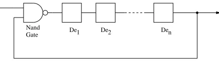
Experimental results. We made a series of experiments on an Altera Stratix II board with a non-well-stabilized switching power supply. We have implemented two different ring oscillatorsR andR′ made up of a NAND gate and the same number of delay elements (see Figure1). The clock signals of the two oscillators are connected to an output PIN and analyzed with a digital oscilloscope at 10 Gigasamples per second.
0 0 1 1
Nand
Gate De1 De2 Den
Fig. 1.Ring oscillator.
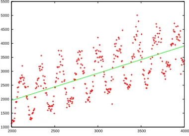
From the data recorded by the oscilloscope we recover two sequences t = (t0, . . . , tn) andt′= (t′0, . . . , t′n′) corresponding to the flipping times of the signals ofRandR′, respectively. We obtained that the mean period ofRis 14,5ns and that ofR′ is 14,7ns. We remark that althoughR andR′ have identical VHDL specifications, their mean periods are not equal because of the variability of routing. Starting from the sequencet= (ti) of flipping times ofR, we compute the estimator Vs(ℓ) from the time gaps (tℓ(i+1)−tℓi). Figure 2 represents the graph of Vs(ℓ) as a function ofℓ.
We remark thatVs(ℓ) is not a straight line with slopes2Xas one might expect if the global deterministic jitters were negligible. The accumulation phenomenon of the Gaussian jitter is nevertheless perfectly visible as the function Vs(ℓ) is globally increasing. We can explain the shape ofVs(ℓ) by introducing a frequency perturbation function α(t) to model the effect of global deterministic jitters. Specifically, assume that the expected value of Tk+1−Tk given thatTk =tk is close to mX
α(tk) where
1
α(t) = 1 +Asin( 2πt
P +B) is sinusoidal of period P with
1000 1500 2000 2500 3000 3500 4000 4500 5000 5500
2000 2500 3000 3500 4000
Fig. 2. Simple measure:Vs(ℓ) as a function ofℓ.
ofα(t) to the variance of the jitter is maximal and we obtain a local maximum of the graph ofVs(ℓ).
3.2 Differential measures
The previous experiments suggest that the statistical models of Section2 may not be accurate in general, for a non-well-stabilized oscillator, due to slow fluc-tuations of the average frequency µ (or equivalently of the half-period mX). This phenomenon naturally leads us to model the phase of such an oscillator by a Wiener process with a non-constant drift of the formµ(t) =µ α(t), where
α(t) > 0 is a perturbation function, intuitively close to 1, and equal to 1 in average.
Alternatively, in terms of flipping times Tk, we may equivalently consider a modified classical model where the i.i.d. variablesXk now represent half-periods that are scaled by α(t). More precisely, to define Tk+1 with respect to Tk and
Xk, the relationXk =Tk+1−Tk is now replaced byXk =
RTk+1 Tk α(t)dt.
Following the empirical conclusions of Valtchanovet al. [16] regarding a de-composition between local and global jitters of oscillators, we expectα(t) to be
global, that is, applicable to all the (similar) oscillators running on a given FPGA, and to haveslow variations compared to the nominal frequency of oscillators.
More precisely, letmX′ be the average half-period ofR′(typically estimated as in Subsection3.1) and let φ be the simplest, continuous, strictly increasing, piecewise-affine function from [t′0, t′n′] to [0, n′] such that φ(t′k) = k mX′ (0 ≤
k≤n′). Assume for simplicity thatt′0≤t0 andtn≤t′n′. We define the rescaled sequenceτ = (τ0, . . . , τn) byτj=φ−1(tj) (0≤j ≤n), that is, more concretely: for everyj,
τj
mX′
=k(j) + tj−t ′ k(j)
t′k(j)+1−t′k(j) (16)
wherek(j) = max{k∈N|t′
k ≤tj}. Finally, we consider the differential estima-torsVd(ℓ) defined by
Vd(ℓ) = ˆV(τℓ−τ0, τ2ℓ−τℓ, . . . , τ⌊n ℓ⌋ℓ−τ(⌊
n
ℓ⌋−1)ℓ). (17)
We note that, by construction, sampling the digital signal corresponding to the flipping times t at times (t′
0, t′2, . . . , t′2⌊n′ 2⌋
) — this is typically done by connecting the outputs of Rand R′ to a type-D flip-flop — would give exactly the same binary outputs as the sampling of the signal corresponding toτ by a clock signal of constant period 2mX′.
As we show in Appendix B, this analogy also applies to Vd(ℓ), that is: ac-cording to the physical assumptions above,Vd(ℓ) should be approximately pro-portional toℓ. More precisely, we show that the proportionality factors2≈Vd(ℓ)
ℓ is an estimation of the amount of local noise available inRandR′, in the sense that
s2≈s2X+
mX
mX′
2
s2X′ (18)
wheremXandsX (resp.mX′ andsX′) are the mean and the standard deviation of the durationsXk related toR (resp.Xk′ related toR′).
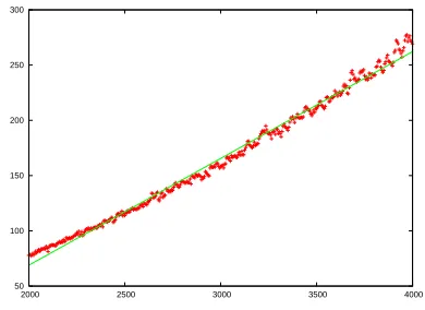
Experimental results. We go on with the experimental results paragraph of Sec-tion3.1with the same experimental device and keep the same notations. From the flipping time sequencest= (ti) andt′ = (t′j) ofRandR′, as described above, we compute the estimatorVd(ℓ) from (τℓ(i+1)−τℓi) in the case of a differential measure.
Figure 3 represents the graph of Vd(ℓ) as a function of ℓ. We can see that the function Vd(ℓ) is well approximated by an affine function. The differential measure has canceled out the influence of the global deterministic jitter. By doing an affine regression onVs(ℓ) we obtain a line with slope 0.97, while in the case ofVd(ℓ) the slope of the linear regression is 0.09. As a consequence, we see that the usual simple measure leads to a gross overestimation of the variance of the jitter ofR.
4
Statistical tests
50 100 150 200 250 300
2000 2500 3000 3500 4000
Fig. 3.Differential measure:Vd(ℓ) a function ofℓ.
experiments require a direct access to the (possibly multiple) ring oscillators be-forethe signal is digitalized. In this section, we build upon the theoretical model presented in Section2, and report higher-level experiments carried out directly on the bit stream of a sampled ring oscillator and applicable to any source that is presumably equivalent.
Our tests are based on the biases predicted by the statistical model when the quality factor Q = σ2∆t (see Section 2) is insufficient, that is, when the sampling rate ∆t1 is too high compared to the amount of noise availableσ2. Such a weakened behavior can be obtained on purpose by accelerating the sampling clock. Interestingly, it could also occur in the case of a bad design or a physi-cal attack on the generator. After discussing a simple auto-correlation test, we present numerical experiments related to the likelihood of a given sample.
4.1 Auto-correlation test
A consequence of Proposition 1 is that the first coefficient of auto-correlation of a sample b= (b1, . . . , bn)∈ {0,1}n defined byc(b) = n−11Pn−j=11(−1)bj+bj+1, gives a statistical test especially well suited to detect biases in the bit-stream of random generators based on oscillators. Indeed, we note that the expectation of
c(b) is 0 on a perfect random source, but amounts to
X
b
c(b)p(b) = 8
π2cos(2πν)e −2π2
Q+O(e−4π2
Q) (19)
on a random generator such as considered in Section2(with the same notations). Besides, on perfect random sources, by the central limit theorem,c(b) approxi-mately follows a centered Gaussian distribution of variance 1
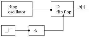
Experimental results. We have implemented a single ring oscillatorRcomposed of 49 inverters on an Altera Stratix II FPGA. We let the oscillatorRbe sampled via a type D flip-flop triggered by a divider applied to the quartz clock signal of the FPGA, running at frequencyf = 50MHz (see Figure4). Using a digital
00 11
00 11 00000 11111
000 111
Ring oscillator
D flip flop
:k
b[t]
Fig. 4.Scheme of the experiment
oscilloscope, we could measure the mean period of the ring oscillator: 2mX = 33.4ns. By performing a differential measure, we also estimated the variance of the jitter per half period ofR to be approximatelys2X = 0.0047ns2. From this, we could estimate the quality factor of the generator for a given division factor
D to be Q ≈ s2X
4m3
X
D f ≈
D
197840. Table 1 shows the empirical auto-correlation factors obtained for various samples. We observe as expected that a too small quality factor causes the source to be immediately discarded as|c(b)| ≫ √1
n.
Division factor (D) Sample size (n) Quality factor (Q) c(b) 1
√ n
2559 71483 0.012 -0.7523 0.003
22598 110621 0.114 0.0020 0.003
40000 62498 0.202 -0.0007 0.004
Table 1.Auto-correlation factorsc(b) for samples from three random sources.
4.2 Maximum likelihood estimation
The auto-correlation test is useful to detect flaws, but is not sufficient to esti-mate the physical parameters of a generator, namely its quality factorQand its frequency ratioν. On the other hand, the techniques used for proving Proposi-tion1 (see SectionAin appendix) make it possible to compute the probability
p(Q, ν,b) of a samplebin function of (Q, ν) efficiently and with good precision. Following the rational of maximum likelihood estimators, we may then choose the two parameters (Q, ν) that maximize the probability of a given sample. Note that the mathematical model of sampling entailsp(Q, ν,b) =p(Q,±ν+k,b) for anyk∈Z. Therefore, we can only observe ¯ν =|(ν+1
2 mod 1)− 1 2| ∈[0,
Numerical experiments. The graphs of Figure 5 result from the evaluation of these probabilities on two bit samples of sizen= 50000: one sample taken from a perfect simulated source (right-hand side), and the other from our FPGA for a division factorD= 22598 (left-hand side). On both graphs,Qis represented on theX-scale,ν on theY-scale, and the plotted value on the Z-scale is log2(1 + 2np(Q, ν,b)). We observe that contrarily to the simulated perfect source, the real
0 0.05
0.1 0.15 0.2 0.25 0.3 0.35
0.4 0.45 0.5 0 0.2 0.4 0.6 0.8 1 0 1 2 3 4 5 6 7 8 9 "output.22598.1MS2__L50000_O60000.dat" 8 6 4 2
0 0.05
0.1 0.15 0.2 0.25 0.3 0.35
0.4 0.45 0.5 0 0.2 0.4 0.6 0.8 1 0 0.2 0.4 0.6 0.8 1 1.2 1.4 "output_uniform_simul__L50000.dat" 1 0.5
Fig. 5.Maximum likelihood estimations.
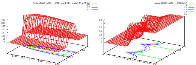
data cause two symmetric peaks indicating plausible values forQandν mod 1. We also carried out the analysis on 1000 bits of the source D = 2559 and on 60000 bits of the source D = 40000 (Figure6, left and right respectively). We observe that the maximum likelihood approach succeeds — that is, clearly
0 0.005 0.01 0.015 0.02 0.025
0.03 0 0.2 0.4 0.6 0.8 1 0 50 100 150 200 250 300 350 "output.2559.1MS2__L1000_xmin0.001_xmax0.03_p20.dat" 300 200 100
0 0.05 0.1 0.15
0.2 0.25 0.3 0.35
0.4 0.45 0.5 0 0.2 0.4 0.6 0.8 1 0 0.2 0.4 0.6 0.8 1 1.2 "output.40000.1MS2__L60000.dat" 1 0.8 0.6 0.4 0.2
Fig. 6.Maximum likelihood estimations (2).
caseD = 2559, we see that global maximum of the plausability function leads to the right value of the quality factor Q ≈ 0.01. The caseD = 22598 is less clear as the plot seems to indicate a quality factor twice as much as the expected value Q= 0.11. However, experiments on simulated sources for Q= 0.15 (see Table 7 below) partly mitigate this impression. Besides, we should emphasize that the estimation of the quality factor Qrelies on a differential measure that filters out global frequency jitters, whereas the graphical test does not.
Further numerical experiments on simulated sources. To study the convergence and the reliability of our graphical estimator, we conducted a number of nu-merical experiments on simulated random sources for different quality factorsQ
and frequency ratioν. In Table 2, we report the amounts of bits that we found usually necessary for a graphical estimation to be conclusive.
Quality factor (Q) Best case (¯ν= 0) Worst case (¯ν= 0.25)
<0.05 <1000 <5000
0.1 50000 100000
0.2 500000 1000000
0.3 2000000 >4000000
Table 2.Typical sample sizes needed by the estimator.
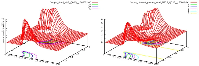
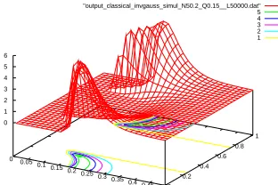
Finally, to validate the equivalence between the different mathematical mod-els (Section 2), we simulated several sources of parameters Q= 0.15 and ν = 50.2, according to the model of Wiener processes and two models of alternating renewal processes using Gamma and Inverse Gaussian laws (see Figure 7 and Figure8). The resulting graphs for 50000 bits of data confirm the intuition that the three sources behave similarly and the fact that the graphs provide correct estimations of the physical parameters.
0 0.05 0.1 0.15
0.2 0.25 0.3 0.35
0.4 0.45 0.5 0 0.2 0.4
0.6 0.8
1 0
2 4 6 8 10 12 14 16 18 20
"output_simul_N0.2_Q0.15__L50000.dat" 15 10 5
0 0.05 0.1 0.15
0.2 0.25 0.3 0.35
0.4 0.45 0.5 0 0.2 0.4
0.6 0.8
1 0
1 2 3 4 5 6
"output_classical_gamma_simul_N50.2_Q0.15__L50000.dat" 5 4 3 2 1
0 0.05 0.1 0.15 0.2 0.25
0.3 0.35
0.4 0.45 0.5 0 0.2 0.4
0.6 0.8
1 0
1 2 3 4 5 6
"output_classical_invgauss_simul_N50.2_Q0.15__L50000.dat" 5 4 3 2 1
Fig. 8.Maximum likelihood estimations (4).
5
Conclusion
We have seen that the family of random bit generators made of a ring oscillator sampled by a clock signal is amenable to a comprehensive statistical study.
On the conception side, we provide practical formulas and an experimental method to control the main security parameters of a TRNG — in particular its entropy rate and the probability biases in the output bits. Incidentally, our experiments give an explanation for the observation reported in the literature that ring oscillators have a tendency to couple with each other. Indeed, there is at least one coupling between ring oscillators by the way of the global deterministic jitters. Some authors [7] conclude that this phenomenon significantly reduces the amount of randomness produced by a TRNG. Our observations tend to show that the global deterministic jitters do not undermine the randomness of a TRNG by itself, but can lead to dangerous overestimations.
On the attackers’ side, we have seen that it is easy to recover the statisti-cal parameters of an oversampled oscillator from a sufficiently large amount of output bits. In extreme cases, we note that this allows one to implement opti-mized brute-force attacks on the unknown output vectors of such a generator. Indeed, one may determine the corresponding distributions and try out the most probable values first (see [10] for a detailed analysis).
Finally, on the performance side, we observe that, in order to achieve a near-to-one quality factor and obtain almost perfectly random bit-sequences, it is necessary to sample the ring oscillator at a very low frequency. Interestingly, our statistical model uncovers some possible approach to improve the throughput of such a TRNG. Indeed, our theoretical study (Proposition 1) suggests that the residual biases of the generator would be considerably lowered if one could lock the term cos(2πν) to a very small value.
based on ring oscillators. For instance, a natural design, presumably more robust to global deterministic jitters [16], consists of a ring oscillator sampled by another ring oscillator — the random bitstream being accommodated to the system clock through a FIFO-stack. As an encouraging result, we have proved using reason-able heuristics (see Appendix C) that such a design can be well approximated by the model considered in this paper for an appropriate choice of parameters. Another common design of generator, motivated by bit-rate efficiency, is made of a (XOR) combination of several ring oscillators before sampling (see for in-stance [14]). Achieving precise and physically-validated security analyses for such complex designs constitutes a challenging open problem.
Acknowledgments. We are very thankful to Fr´ed´eric Valette for his support to this project and for his contributions to the physical experiments. Our work also greatly benefited from early discussions with S´ebastien Kunz-Jacques, who brought the idea of using specific statistical tests, and with Jean-Michel L´evy-Bruhl, who suggested the need for a simpler mathematical model.
References
1. A statistical test suite for random and pseudorandom number generators for cryp-tographic applications. NIST Special Publication (SP) 800-22 rev. 1, 2008. Avail-able athttp://csrc.nist.gov/CryptoToolkit/tkrng.html.
2. A. Abcunas, C. Coughlin, G. Pedro, and D. Reisberg. Evaluation of random num-ber generators on FPGA’s. Technical report, Worcester Polytechnic Institute, 2004.
3. Holger Bock, Marco Bucci, and Raimondo Luzzi. An offset-compensated oscillator-based random bit source for security applications. InCHES, pages 268–281, 2004. 4. W. Coppock and C. Philbrook. A mathematical and physical analysis of circuit jitter with application to cryptographic random bit generation. Technical report, Worcester Polytechnic Institute, 2005.
5. David Roxbee Cox and Hilton David Miller. The Theory of Stochastic Processes. CRC Press, 1977.
6. Alper Demir, Amit Mehrotra, and Jaijeet Roychowdhury. Phase noise in oscilla-tors: a unifying theory and numerical methods for characterisation. InDAC ’98: Proceedings of the 35th annual conference on Design automation, pages 26–31, New York, NY, USA, 1998. ACM.
7. Markus Dichtl and Jovan Dj. Golic. High-speed true random number generation with logic gates only. InCHES, pages 45–62, 2007.
8. Michael Epstein, Laszlo Hars, Raymond Krasinski, Martin Rosner, and Hao Zheng. Design and implementation of a true random number generator based on digital circuit artifacts. InCHES, pages 152–165, 2003.
9. Wolfgang Killmann and Werner Schindler. A design for a physical RNG with robust entropy estimators. InCHES, pages 146–163, 2008.
10. John Pliam. The disparity between work and entropy in cryptology. Cryptology ePrint Archive, Report 1998/024, 1998. http://eprint.iacr.org/.
12. Werner Schindler and Wolfgang Killmann. Evaluation criteria for true (physical) random number generators used in cryptographic applications. In CHES, pages 431–449, 2002.
13. C. E. Shannon. A mathematical theory of communication. Bell System Tech. J., 27:379–423, 623–656, 1948.
14. B. Sunar, W. J. Martin, and D. R. Stinson. A provably secure true random number generator with built-in tolerance to active attacks. IEEE, 2007.
15. Henk C. Tijms. A first course in stochastic models. Wiley, 2003.
16. B. Valtchanov, A. Aubert, F. Bernard, and V. Fischer. Modeling and observing the jitter in ring oscillators implemented in FPGAs. In11th IEEE Workshop on Design and Diagnostics of Electronic Circuits and Systems, pages 1–16. IEEE, 2008.
A
Computing probabilities and source entropy
This section provides the mathematical justifications and additional details re-lated to Section2.
A.1 Exact expression of probabilities by means of Fourier series Fourier coefficients of ϕ(t). From the point of view of an outside observer, the state of the generator at a given timetcorresponds to a certain probability measure on the phaseϕ(t).
More precisely, let pt(x | ξ) be the density of probability (possibly a dis-tribution) of ϕ(t) after a certain experiment described by precondition ξ. We introduce the Fourier coefficients ofpt(x|ξ):
ct(k|ξ) =
Z +∞
−∞
pt(x|ξ)e−2πikxdx (20)
for everyk∈Z.
Remark 4. We note that ct(0|ξ) =
R+∞
−∞ pt(x|ξ)dx= 1.
Remark 5. The reason why we restrict k to integer values is that we are only interested in the probability measure ofϕ(t) =ϕ(t) mod 1, which is described by the 1-periodic density function:
pt(x|ξ) =
X
k∈Z
pt(x+k|ξ) (21)
Indeed we observe that
ct(k|ξ) =
X
u∈Z
Z 1
0
pt(x+u|ξ)e−2πikxdx (22)
=
Z 1
0
pt(x|ξ)e−2πikxdx (23)
Assuming that the inverse formula for Fourier series holds forct(k|ξ), we obtain:
pt(x|ξ) =
X
k∈Z
Effect of time evolution. The following lemma expresses the effect of time evolution on the Fourier coefficient of a density of probabilitypt(x|ξ).
Lemma 1. Assume an average drift speed µ and volatility σ2 (σ > 0) for the Wiener process ϕ(t). For any t0 ≤ t and for every precondition ξ concerning
only events prior to t0, we have
ct(k|ξ) =ct0(k|ξ)e−2πiµ(t−t0)ke−2π 2
σ2(t−t0)k2
(25)
Proof. Letf(x) = 1
σ√2π(t−t0) exp
−(x−µ(t−t0))2
2σ2(t−t0) be the density probability of the Gaussian distribution with meanµ(t−t0) and varianceσ2(t−t0). By construction of Wiener processes (Eq. 1), we have that pt(x|ξ) =pt0(x|ξ)∗f(x) where∗ denotes the convolution product. The result then follows from the property of Fourier transform w.r.t. convolution, and the computation of Fourier coefficients
for normal distributions. ⊓⊔
Notation. Letct(ξ) denote the infinite vector (ct(k|ξ))k∈Z. Letδkbe the Dirac (infinite) column vector with a one in k-th position, andπj be Dirac (infinite) row vector with a one inj-th position.
The linear relation above is written
ct(ξ) =E[t−t0]ct0(ξ) (26)
whereE[t−t0] denotes the (t−t0)-evolution operatorwith coefficient (j, k)∈Z2 given by:
πjE[t−t0]δk =
(
0 ifj6=k
e−2πiµ(t−t0)k e−2π2σ2(t−t0)k2 otherwise ifj =k (27)
Remark 6. Let1= (1)k∈Z denote the vector made of ones. We note thatσ >0 implies that for anyt >0,kE[t]1k1<∞.
Effect of sampling. The next lemma expresses the effect of sampling a bitb
on the Fourier coefficient of a densitypt(x|ξ).
Lemma 2. For anyt and for every preconditionξconcerning only events prior tot, we have
ct(j|ξ, s(t) =b) = 1
P
X
k∈Z
γb(j−k)ct(k|ξ) (28)
whereγb(k) =R01gb(x)e−2πikxdx is thek-th Fourier coefficient of the (periodic)
sampling probability gb, and
P =P[s(t) =b|ξ] =X k∈Z
Proof. By definition and by Bayes formula on probability densities, we have
pt(x|ξ, s(t) =b) = 1
P pt(x|ξ)gb(x)
where
P =P[s(t) =b|ξ] =
Z +∞
−∞
pt(x|ξ)gb(x)dx
The result follows from the usual property of Fourier coefficients, which trans-form products into convolutions, and maps mean values of functions to their
0-th coefficients. ⊓⊔
Notation. The relation above is written
ct(ξ, s(t) =b) = 1
P S[b]ct(ξ) (30)
whereS[b] denotes theb-sampling operator with coefficient (j, k) given by
πjS[b]δk=γb(j−k) (31)
andP =π0S[b]ct(ξ).
Exact expressions of the probabilities. We may now determine the proba-bilities of sampling arbitrary bit patterns from a jittered oscillator.
Proposition 3. Let A0 =e−2πiµ andB0=e−2π 2σ2
. For any x∈R, let 1x= (e−2iπkx)
k∈Z. Using the other vector notations above, we have for every t >0,
p1,x(t) = P[s(t) = 1|ϕ(0) =x] (32)
= π0S[1]E[t]1x (33)
= X
k∈Z
γ1(−k)e−2iπkxAtk0 Btk 2
0 (34)
and for everyt1< t2< . . . < tn, lettingi0=in= 0, we have
fb(t) = P[s(t1) =b1, . . . , s(tn) =bn] (35) = π0S[bn]E[tn−tn−1] . . . S[b2]E[t2−t1]S[b1]δ0 (36)
= X
(i1, ..., in−1)∈Zn−1 n−1
Y
k=0
γbk(ik−ik+1)A
Pn−1
k=1ik(tk+1−tk)
0 B
Pn−1
k=1i 2
k(tk+1−tk)
0
(37)
Proof. We observe that
p1(t) = P[s(t) = 1|ϕ(0) =x]
= π0S[b]ct(ϕ(0) =x) by Lemma2 = π0S[b]E[t]c0(ϕ(0) =x) by Lemma1
= π0S[b]E[t]1x by definition of Fourier coefficientsct(k|ϕ(0) =x) Similarly, lettingqn=P[s(t1) =b1, . . . , s(tn) =bn], we have for all n >0
qnctn(s(t1) =b1, . . . , s(tn) =bn)
= qn
Pn
S[bn]ctn(s(t1) =b1, . . . , s(tn−1) =bn−1)
= qn−1S[bn]ctn(s(t1) =b1, . . . , s(tn−1) =bn−1)
= qn−1S[bn]E[tn−tn−1]ctn−1(s(t1) =b1, . . . , s(tn−1) =bn−1) = S[bn]E[tn−tn−1] qn−1ctn−1(s(t1) =b1, . . . , s(tn−1) =bn−1)
wherePn=P[s(tn) =bn |s(t1) =b1, . . . , s(tn−1) =bn−1].
Given thatq0ct0() =δ0andE[t1−t0]δ0=δ0, we obtain by induction onn:
qnctn(s(t1) =b1, . . . , s(tn) =bn)
=S[bn]E[tn−tn−1] . . . S[b2]E[t2−t1]S[b1]δ0 The first expression offb(t) follows fromπ0ct(ξ) =ct(0|ξ) = 1.
In the end, we obtain the desired final expressions by expanding the matrix products (the conditionsσ >0,t >0 andt1< . . . < tn ensuring that every sum
is absolutely convergent). ⊓⊔
A.2 Approximate expressions of probabilities and entropy
Consider the functiong1(x) defined in Section2. The Fourier coefficient ofg1(x) are given by
– γ1(0) = 12;
– for everyk6= 0,γ1(2k) = 0; and – for everyk,γ1(2k+ 1) = (2k+1)πi .
Fromg0+g1= 1, we also deduce thatγ0(0) = 12 andγ0(k) =−γ1(k) fork6= 0. In particular, the exact expression ofp1,x(t), taken from Proposition3, becomes
p1,x(t) =
X
k∈Z
γ1(−k)e−2πik(µt+x)e−2π 2
σ2tk2 (38)
= 1 2−
2
π
+∞
X
N=0
sin(2π(µt+x)(2N+ 1))
2N+ 1 e
−2π2
σ2t(2N+1)2
(39)
B=B∆t
0 =e−2π 2
Qandi
0=in= 0. The exact expression ofp(b) =fb(t), taken from Proposition3, becomes
p(b) = X
(i1, ..., in−1)∈Zn−1 n−1
Y
k=0
γbk(ik−ik+1)A
Pn−1
k=1ik B
Pn−1
k=1i 2
k (40)
= +∞
X
N=0
aN(b)BN (41)
where
aN(b) =
X
Pn−1
k=1ik2=N
n−1
Y
k=0
γbk(ik−ik+1)A
Pn−1
k=1ik. (42)
From the expressions of γ0(k) and γ1(k), we obtain in particular the first termsaN(b):
a0(b) = 1
2n (43)
a1(b) = γb1(−1)γb2(1)γb2(0) . . . γbn(0)A
+ γb1(0)γb2(−1)γb3(1) . . . γbn(0)A
+ . . .
+ γb1(0) . . . γbn−2(0)γbn−1(−1)γbn(1)A
+ γb1(+1)γb2(−1)γb2(0) . . . γbn(0)A−
1
+ γb1(0)γb2(+1)γb3(−1) . . . γbn(0)A−
1
+ . . .
+ γb1(0) . . . γbn−2(0)γbn−1(+1)γbn−1(−1)A−
1 (44)
= A+A− 1 2n−2π2
n−1
X
j=1
(−1)bj+bj+1
(45)
= 8
2nπ2cos(2πν)
n−1
X
j=1
(−1)bj+bj+1
(46)
We now address the development ofHn=−Pb∈{0,1}np(b) log2p(b). Given that (1 +x) ln(1 +x) =x+P+∞
N=2 (−1)N
N(N−1)xN for|x|<1, and that p(b) tends toa0(b) =21n whenB →0, we have for sufficiently small values ofB:
−p(b) log2(p(b)) =np(b)− 1 2nln(2)(2
np(b)) ln(2np(b)) (47)
=np(b)−2nln(2)1 +∞
X
N=2
(−1)N
N(N−1)ǫ(b)
where we use ǫ(b) = 2np(b)−1 to denote the bias of a vector b. Using that
P
b∈{0,1}np(b) = 1 anda0(b) = 21n, we obtain
Hn=n− 1 2nln(2)
X
b∈{0,1}n
+∞
X
N=2
(−1)N
N(N−1) +∞
X
M=1 2na
M(b)BM
!N
(49)
=n−2n− 1
ln(2)
X
b∈{0,1}n
a1(b)2B2+O(B3) (50)
But, by the previous expression ofa1(b), we have
X
b∈{0,1}n
a1(b)2= 64 22nπ4cos
2(2
πν) X b∈{0,1}n
n−1
X
j=1
(−1)bj+bj+1
2
(51)
= 64
22nπ4cos 2(2
πν) 2n(n−1) (52)
= 64(n−1) 2nπ4 cos
2(2πν) (53)
Therefore, we may conclude that Hn = n−
32(n−1)
π4ln(2) cos 2(2
πν)B2+O(B3).
A.3 Safe bounds on bias and entropy
The proof of Corollary1 runs as follows.
Proof (of Corollary1).By definitionHn=H(s((n−1)∆t), . . . , s(∆t), s(0)) and we have that
Hn+1−Hn =H(s(n∆t)|s((n−1)∆t), . . . , s(∆t), s(0)) ≥H(s(n∆t)|ϕ((n−1)∆t)
=H(s(∆t)|ϕ(0))
=
Z 1
0
H(s(∆t)|ϕ(0) =x)dx
but
H(s(∆t)|ϕ(0) =x) = 1−1 +2 ǫlog2(1 +ǫ)− 1−ǫ
2 log2(1−ǫ)
= 1− ǫ 2
2 ln(2)+O(ǫ 3)
whereǫ= 2P[s(∆t) = 1|ϕ(0) =x]−1 = 4
πsin(2π(ν+x))e− 2π2
Next, we give a proof of Proposition2.
Proof (of Proposition 2).Using the expression ofp(b) at Equation (42) and the fact thatγb(0) = 12, we have that
ǫ(b) = 2np(b)−1 (54)
= X
(i1, ..., in−1)6=0 n−1
Y
k=0
(2γbk(ik−ik+1))A
Pn−1
k=1ikBPnk=1−1i 2
k (55)
Since|A|= 1,B >0 and for everyk, |γb(k)| ≤ 12, we obtain
|ǫ(b)| ≤ X (i1, ..., in−1)6=0
BPnk=1−1i 2
k = ϑ(B)n−1−1 (56)
The lower bound ofHn results the fact that the functionx7→xlog2xis mono-tone:
−p(b) log2(p(b)) =np(b)− 1 2n(2
np(b)) log
2(2np(b)) (57) ≥np(b)−21nϑ(B)n−1log2ϑ(B)n−1 (58)
Hence, by summing onb, we haveHn ≥n−ϑ(B)n−1log2(ϑ(B)n−1)≥n−2. ⊓⊔
B
Physical justifications of differential measures
The goal of this section is to justify that the physical assumptions of Subsec-tion3.2 impliesVd(ℓ)≈ℓ s2 for some values2 that we relate to the amount of noise available inR andR′.
In line with Subsection 3.2, for simplicity, we directly model the flipping timesTk ofRand assume the variablesXk=
RTk+1
Tk α(t)dtto be i.i.d. according
to some distribution of meanmX and standard deviationsX. We modelR′in a similar way using the corresponding prime symbols.
The physical assumptions of our models are the following:
(i) sX ≪mX (small local jitters forR), (ii) sX′ ≪mX′ (small local jitters forR′), and
(iii) α(t)≈1 (small deterministic perturbations onR andR′). (iv) |α′(t)| ≪ m1X and|α
′(t)| ≪ 1
mX′ (slow variations ofα(t)). Note that the last assumption implies that the equationXk =
RTk+1 Tk α(t)dt
can be simplified into
Tk+1−Tk≈
Xk
α(Tk)
(59)
Following the notations of Subsection 3.2, from the two sequences of times t= (t0, . . . , tn),t′ = (t0′, . . . , t′n′), we define a rescaled sequenceτ = (τ0, . . . , τn) such that for everyj (t′0≤tj< t′n′),
τj
mX′
=k(j) + tj−t ′ k(j)
t′
k(j)+1−t′k(j)
, (60)
wherek(j) = max{k∈N|t′ k≤tj}.
To show thatVd(ℓ) = ˆV(τℓ−τ0, τ2ℓ−τℓ, . . . , τ⌊n ℓ⌋ℓ−τ(⌊
n
ℓ⌋−1)ℓ) is
approxi-mately proportional to ℓ, we argue that eachτj+1−τj independently follows a distribution with meanm≈mX and variances2≈s2X+
mX
mX′
2
s2 X′. Indeed, by definition, we have
τj+1−τj
mX′
= tj+1−t ′ k(j+1)
t′
k(j+1)+1−t′k(j+1)
+k(j+ 1)− tj−t ′ k(j)
t′
k(j)+1−t′k(j)
−k(j) (61)
= tj+1−t ′ k(j+1)
t′
k(j+1)+1−t′k(j+1) +
k(j+1)−1
X
k=k(j)
t′ k+1−t′k
t′ k+1−t′k
+ t
′ k(j)−tj
t′
k(j)+1−t′k(j)
.(62)
For all 0≤k≤n′−1, let
ǫ′k= α(t ′
k) (t′k+1−t′k)
mX′ −
1. (63)
By Equation (59) and assumption (ii),ǫ′k approximately follows a centered Gaussian distribution of variance s
2
X′ m2
X′ ≪1. As a consequence, we may write
mX′ (t′
k+1−t′k)
= α(t′k) 1 +ǫ′ k
≈α(t′k) (1−ǫ′k). (64)
By assumption (iv), for k(j) ≤ k ≤ k(j+ 1), a first-order approximation of α(t′k) is α(tj). Therefore, putting altogether (62) and (64) and neglecting second-order terms, we have
τj+1−τj≈α(tj) (tj+1−tj) − α(t′k(j+1))ǫk(j+1)′ (tj+1−t′k(j+1))
−
k(j+1)−1
X
k=k(j)
α(t′k)ǫ′k(t′k+1−t′k)
− α(t′k(j))ǫk(j)′ (t′k(j)−tj).
(65)
We note that the first part of the equation approximately follows a Gaussian distribution of mean mX and variance s2X, whereas the second half approxi-mately (and independently) follows a centered Gaussian distribution of variance (sX′
mX′) 2m2
X. Therefore, we may conclude that the (τj+1−τj) are independent out-comes of a Gaussian distribution of meanmXand variances2=s2X+s2X′(
mX
C
Equivalent physical parameters of a dual-oscillator
TRNG
In Section2, we considered the sampling of an oscillatorR by a perfectly stabi-lized clock signal. The present section is devoted to the study the sampling of an oscillatorR by another ring oscillatorR′. We also allow small global variations of frequency forR andR′ as considered in Section3. Our goal is to show that such a complex system is still well approximated by the simple framework of Section 2.
Model and physical assumptions. We model the phase of the sampled oscillatorR
by a Wiener process of variable speed µ(t) = µ α(t) and volatility σ2. As for the sampling oscillator R′, for simplicity, we directly model the flipping times
Tk and assume the variables Xk =RTTkk+1α(t)dt to be i.i.d. according to some distribution of meanmX and standard deviationsX. (Here we omit the prime symbols for readability.)
As before, the physical assumptions of our models are the following:
(i) σ2≪µ (small local jitters forR),
(ii) sX ≪mX (small local jitters forR′), and
(iii) α(t)≈1 (small deterministic perturbations onR andR′).
(Note that we do not assumeα(t) to have low frequency variations, here.) To compare this setting with the simpler model of Section2, we proceed in two steps. First, we generalize the method used in AppendixAto reason about the effect of time evolution on phases. Second, we use the physical assumptions above to argue that the sampling ofR byR′ can be well approximated by the sampling of a single oscillatorR′′by a periodic time reference, that is, following the model initially considered in Section 2.
Phase evolution revisited. In Appendix A, we noticed that, for an oscillatorR
with constant statistical parametersµand σ2, the evolution of the conditional distribution of the phase from time tk to time tk+1 ≥ tk is expressed by a convolution product:
ptk+1(x|ξ) =ptk(x|ξ)∗fµ(tk+1−tk),σ2(tk+1−tk)(x), (66)
where fm,s2(x) = 1 s√2π exp
−(x−m)2
2s2 is the density function of the Gaussian distribution with meanm and variances2, and ξdenotes any event related to the sampling ofR at times beforetk.
In the case of non constant statistical parametersµ(t) andσ2(t) forR, this equation generalizes as follows:
ptk+1(x|ξ) =ptk(x|ξ)∗fm,s2(x), (67)
wherem=Rtk+1
tk µ(t)dt ands
2=Rtk+1 tk σ
Now let us consider that the sampling timestk are probabilistic drawings of random variables T2k modeling the raising times of another oscillator R′ such that the durations Xk =RTTkk+1α(t)dt are i.i.d. following some densitypX. Be-sides, assume that µ(t) =µα(t) andσ2(t) =σ2α(t) for some constantµand σ. We have that
P[s(T2(k+1)) = 1|ξ] =
Z +∞
−∞
P[s(t) = 1|ξ]dPT2(
k+1)|ξ(t) (68)
=
Z +∞
−∞
g1(x)pk+1(x|ξ)dx, (69)
where we let pk+1(x|ξ) =R pt(x| ξ)dPT2(k+1)|ξ(t) denote the average condi-tional density of the phase ofR at the (k+ 1)-th sampling time.
By definition ofT2(k+1) and from Equation (67), we obtain that
pk+1(x|ξ) =pk(x|ξ)∗g(x)∗g(x), (70) whereg(x) =R∞
0 pX(y)fµy,σ2y(x)dy. Altogether, Equations (69) and (70) allow one to define modified operatorsS[b] andE[t] operating on the Fourier coefficient of pk(x | ξ) similarly as for the proof of Proposition 3. We now argue that in the physical cases under consideration, these new operators are in fact well approximated by the same operators as before, using suitable parameters.
Interpretation. Above, we have let σ2(t) = σ2α(t) instead of σ2(t) = σ2 in the model of Section3.2. This approximation is justified by the assumptions (i) and (iii) that σis small andα(t)≈1.
Formula (70) is similar to Equation (66) except that the Gaussian density is replaced by a function g(x)∗g(x) obtained by averaging the durations between two sampling times. We note that the two formulas are exactly equivalent when
X = ∆t
2 with probability 1: indeed g(x)∗g(x) =fµ∆t,σ2∆t(x). When X has a very small variance (assumption (ii)),g(x)∗g(x) will be very close to a Gaussian function, and therefore we can approximate the behavior of the two composed oscillators by a single one.
More precisely, we compute the mean and the variance of the approximation ofg(x)∗g(x) as follows. LetmXands2X be the mean and the variance ofX. By assumption (ii),sX ≪mX, therefore, lettingf(x, y) =fµy,σ2y(x), we have the following approximation:
g(x) =
Z ∞
0
pX(y)f(x, y)dy (71)
≈
Z ∞
0
pX(y)
f(x, mX) + (y−mX)
∂f
∂y(x, mX)
+ (y−mX) 2 2
∂2f
∂y2(x, mX)
dy (72)
=f(x, mX) +
s2X
2
∂2f
Given thatf(x, y) is infinitely derivable and for every i, j, k ≥0, for every y0, |xk ∂i+jf
∂xiyj(x, y)|is bounded by a summable function ofx, in the neighborhood of
y0, we may compute the first central moments ofg(x) as follows:
Z +∞
−∞
x g(x)dx≈
Z +∞
−∞
x f(x, mX)dx+
s2 X 2
Z +∞
−∞
x∂
2f
∂y2(x, mX)dx (74)
=µ mX+
∂2
∂y2
Z +∞
−∞
xf(x, y)dx
y=mX
(75)
=µ mX+
∂2µ y
∂y2
y=m
X
(76)
=µ mX. (77)
Z +∞
−∞
x2g(x)dx − (µ mX)2≈
Z +∞
−∞
x2f(x, mX)dx − (µ mX)2
+s 2 X 2
Z +∞
−∞
x2∂
2f
∂y2(x, mX)dx (78)
=σ2mX+
s2X
2
∂2 ∂y2
Z +∞
−∞
x2f(x, y)dx
y=mX
(79)
=σ2mX+
s2X
2
∂2(µ2y2+σ2y)
∂y2
y=m
X
(80)
=σ2mX+s2Xµ2. (81)
These values must be doubled forg(x)∗g(x). Finally, we obtain that the com-position of R and R′ by means of a type-D flip-flop is equivalent to a system made of single oscillatorR′′ sampled by a time reference, with frequency ratio