Title: Cubic Spline Based Path Planning for UAV

Available Online atwww.ijcsmc.com

International Journal of Computer Science and Mobile Computing

A Monthly Journal of Computer Science and Information Technology

ISSN 2320–088X

IMPACT FACTOR: 6.199

IJCSMC, Vol. 8, Issue. 12, December 2019, pg.80 – 95

Cubic Spline Based Path

Planning for UAV

Dr. Mohammed Sahib Mahdi Altaei; Ala’a Hassan Mahdi

Computer Science Department, College of Science, Al-Nahrain University, Baghdad, Iraq Computer Science Department, College of Science, Al-Nahrain University, Baghdad, Iraq

[email protected]; [email protected]

Abstract— The problem of path planning for auto-navigating aerial vehicle is handled based on cubic spline (CS) method. For comparison, digital differential analyzer (DDA) method is also used to compute the amount of acceptable deflection of the flight route when it is planned by these methods. This problem require to design a control system for guiding the unmanned aerial vehicle (UAV) along the intended route, and then establish an electronic circuit of such controller. A simple model of quadcopter is used to play the role of UAV with the designed controller to implement a number of practical tests with different flight situations: once using DDA method and another using CS one. The recorded results showed that the deflection percent of the planned path using DDA planning method was about 31%, while it was about 8% for CS method. It is shown that the CS method serves the subject of flight path planning due to less path deflection and smooth flight path are achieved.

Keywords— cubic spline, path planning, unmanned aerial vehicle, Digital Differential Analyzer, Ground Station

1. Introduction

changed. The controller has the ability to alter the desired navigation, where the proportional integral derivative (PID) algorithm in the controller restores the actual navigation parameter to the desired value in the optimum way, with minimal delay or overshoot, by controlling the power output of the rotors motors [3].

This paper handle the problem of flight controlling, command introducing, and communications protocols to establish a useful planned path for determining the flight map. The planned path is then simulated to ensure the correct achievement of present work.

2. Aircraft Mobility

Robotic aircraft starts with studying physical motions to model successful robot's movements, which is a process that leading to determine the requirements and effecting parameters on the targeted system, such as aircraft forces, degree of freedom (DoF), navigation parameters, and flight parameters [4]. Four forces affect the aircraft while flying, they are: thrust, drag, lift, and weight as shown in Figure (1). Thrust is a reaction force described quantitatively by Isaac Newton's second and third laws. “When a system expels or accelerates mass in one direction, the accelerated mass will cause a force of equal magnitude but opposite direction on that system”. Drag is a force that

acting opposite to the relative motion of aircraft motion. Lift is a force

generated when air flowing past the surface of a body which is the component of the force parallel to the flow direction. Lift conventionally acts in an upward direction in order to counter the force of gravity. Weight is the force generated by the gravitational attraction of the Earth on the aircraft [5].

Figure (1) Directions of the four forces Thrust, drag, lift and weight [6].

Figure (2) Aircraft 6-DOF [6].

The translation in three perpendicular axes, combined with changes in orientation through rotation about three perpendicular axes, often termed yaw (normal axis), pitch (lateral axis), and roll (longitudinal axis) of the aircraft fuselage at the center of gravity (COG) of the aircraft. The roll is the motion along a straight horizontal line that passes through the nose to the tail of the aircraft fuselage at the CoG of the aircraft, any aircraft fuselage movement around the X-axis will cause a rotation; the angular deference in rotation direction (ΔR) is the Roll angle. Aircraft nose movement around the Z plane will cause deference in the aircraft angular heading direction, the deference in heading direction (ΔH) is rolling or yawing. While the pitch is the motion along a straight horizontal line that passes through the right to the left side of the aircraft fuselage at the CoG of the aircraft, any aircraft fuselage movement around the Y axis will cause a rotation, the angular deference in rotation direction (ΔP) is the Pitch angle [8].

Figure (3) shows the instantaneous position of aircraft that used to specify the geographical location of aircraft on Earth. Three positioning axes are

considered, they are: Longitude, Latitude, and Altitude (or X, Y, and Z

frequently). The longitude and latitude are angles that uniquely define points on a sphere. Together, the angles comprise a coordinate scheme that can locate or identify geographic positions on the surfaces of Earth; while altitude defines the height of the object above the surface of Earth [9].

3. Air Navigation Positioning

In air navigation, waypoints most often consist of a series of abstract Geographical positioning system (GPS) points that create artificial airways are called sky highways that created specifically for purposes of air navigation. In addition to flight conditions, waypoints are predetermined and stored in the navigation map before the flight trip to be started. Waypoint is an intermediate point or place on planned route, it requires presenting the latitude, longitude and altitude of the current or targeting location. Aircraft detects its position by GPS and then determine the deflection from the planned path as shown in Figure (4), and then according to the amount of the deflection it corrects its actual path. Therefore, waypoints refer to coordinates that specify one position on the planned path that is generally determined computationally [10]. The use of waypoints connotes to the determination of reference point in physical space,

most often associated with navigation. The longitudinal

and latitudinal coordinate of GPS point are mapped into other entity, which is a fixed geographical point such as an airport. When such a point corresponds to an element of physical geography on land, it can be referred to as reference landmark [11]. Aircraft can move on straight path connecting two waypoints, but turning to any direction cannot be suddenly occurred due to the sharp turn may cause a threat to the aircraft. In order to avoid such turns and generate a smooth turning path, path planning technique is used in primary stage to determine the map of the airplane route from the start station into the destination point passing through many waypoints. Figure (5) shows two methods to determine the planned path, the first necessitate the aircraft to pass through all waypoints, while the second necessitate the aircraft to move in smooth actual path and passing through same waypoints [12].

Figure (4) Navigation positioning determination [12].

Computer simulation is an imitation operation required to develop a model for testing the planned path. This model related to the behavior of the aircraft over time. The simulation based navigation is used for the performance optimization, safety, training and testing. Simulation is used when the real aircraft cannot be engaged, because it might be exposed to danger at the flight. The simulation results are then compared to the experimental results to improve the behavior of the used mathematical model. The key issues in simulation include acquisition of valid source information about the relevant selection of key characteristics and behaviors, the use of simplifying approximations and assumptions within the simulation, and fidelity and validity of the simulation outcomes. Procedures and protocols for model verification and validation are an ongoing research and development in simulations technology [13].

4. Related Works and Contribution

There are many literatures found in the field of path planning, some of them are concerned with designing the aerial map without explanation of how determining the way points of the aerial planned path. The important related works that discussing such interest point besides our contribution are mentioned in the following subsections.

4.1 Related Work

There is a great deal of focus was granted to auto navigation systems and simulation. Numerous approaches were developed in order to achieve more efficient techniques for serving applications in the field of interest. The most significant literatures are mentioned in the following with details:

1. Jun M., and Andrea R. in 2003 proposed a path planning algorithm based

on a map of the probability of threats, which can be built from a priori surveillance data. The proposed approach was successful when applied on different actual cases. It was used to planning the path of the airplane toward the destination point with smooth path without the necessity to pass across middle way points [14].

2. Mahdi M. S. in 2007 analyzed the airplane mobility to develop an

airplane navigation model, this model is used to estimate the planned path of the auto-navigation control system that tested by the simulation technique to present the behavior of the navigation parameters. The model was improved by taking in account the atmospheric effects on the airplane mobility and determining the route deflection due to suddenly effects of atmosphere [4].

3. Haque S., and et. al. in 2017 designed a flight microcontroller is used in

telemetry data as well as the important weather parameters. There was a predefined fly zone of is determined for the drone in the GCS, the controller was enables to compute the planned path and guide the airplane near or fit the flight situations [15].

4. Monwar M., and et. al. in 2018 suggested a novel path planning

algorithm, which is proposed for performing energy-efficient inspection, under stringent energy availability constraints for each UAV. This method showed efficiency to decide the planned path toward the destination point in shorter path without need to pass across the way points along the desired path, the practical test showed reduce distance and time till reaching the target point [16].

5. Shi Z., and Keong W. in 2018 proposed a collision-free path planning

algorithm that is based on A* algorithm. The main novelty is that they invent a heuristic function that also considers waiting time. Implementation of this algorithm simulates UAV delivery using Singapore's airspace structure, their simulation exhibits desirable runtime performance. The use of the proposed algorithm showed a decrease in the percentage of collision-free routes when increases the number of requests per unit area, and this percentage drops significantly at boundary values [17].

4.2 Our Contribution

In UAV project, landing and gaining altitude are well challenges to the controller. The nonlinear flight controller suffers from huge performance degradation whenever the UAV leaves the hovering conditions to perform aggressive maneuvers. Actually, the design of flight controller is still the monopoly of the manufactured companies and it regarded as one of its work secrets. Path planning is the most interesting topic in the designing stage. The researches are still under way to propose and design an autonomous navigator to be able to reach accurate flight without exposed to accidents. The main objective is accurately deriving the UAV into destination point with safe and different flight situations of taking-off, hovering, flight, and landing. The simulation technique is used to test the control process against such flight situations, the use of cubic spline method for path planning of the flight route help to successfully achieve the safe situations of UAV during the flight.

5. Proposed Controlling Method

on UAV. The controller receives the start order from the GS, and then orders the simulator to sense the flight situations periodically. At each control interval, the controller receives sensors data and determines the error occurs in the flight situations in terms of planned path, these errors are deflections from the intended situations. Accordingly, correction commands are estimated based on determined deflections and exported to the control tools to guide the airplane toward the desired situations. These commands have values equal to the deflections but in opposite direction. This auto navigation process continues guiding the UAV toward the intended route and desired situations, where the amount of deflection is reduced time by time. The following subsections explain more details about path planning and control process:

Figure (6) Generic structure of used controller.

5.1 Planned Path Determination

Table (1) Input database of flight map and intended situations.

Way Points

Position

Speed (m/h)

RD

(m)

X(m) Y(m) Z(m)

1 89 185 8 20 1

2 42 112 6 20 1

3 122 67 9 20 1

4 245 80 10 20 1

5 259 160 10 15 1

6 170 105 10 15 1

7 136 246 6 18 1

The last column in Table (1) is the radius of arrival (RD), which helps the

controller to determine the time of switching to the next way point. The process

of switching is done by comparing the distance RD between the current position

(xc, yc) on the actual route and the target way point (x2, y2) with the radius of

arrival of the target way point. If RD is less than the radius of arrival then the

airplane is considered arrived to the end of current route segment (reach the area of the target way point). Therefore, the controller should switch with the next way point within the planned route due to the airplane is actually reaching the arrival area of the next way point of the predefined radius of arrival.

5.2 Actual Path Determination

Path Planning is the most important phase in building an autonomous embedded navigator system. Two methods are getting the interest to be used for drawing the planned path of the aircraft on air; they are DDA method and CS method. The DDA method determines normal lines connecting each two waypoints, while CS method determines curved line connecting each two waypoints. Both interested methods are passing through multiple waypoints as shown in Figure (7) [18]. More details about DDA and CS are given in the following subsections:

Figure (7) DDA path determination versus CS path [18].

5.2.1 DDA Method

simplest implementation of DDA, in which the DDA algorithm interpolates the

values of yi in interval for each xi according to the following equations;

Algorithm (1) lists the sequential steps of the DDA method [19]:

xi = xi−1 + 1 … (1)

yi = yi−1 + m … (2)

where

Δx = xend − xstart … (3)

Δy = yend − ystart … (4)

m = Δy/Δx … (5)

where, xi and yi are components of current position, xs, xe, ys, and ye are

components of start and end position for specific route segment, and m is the number of division of that route segment.

Input ( , ) and ( , ) \\ start and end points.

Output ( , ) \\ generated point on the line.

Procedure:

End

M= /

if >

else

End if

=

=

Loop For to

= =

Plot ( , ) = +

= +

End Loop

5.2.2 Cubic Spline Method

Cubic spline (CS) method is a spline constructed of piecewise third

order polynomials which pass through a set of control points. The

second derivative of each polynomial is commonly set to zero at the endpoints,

since this provides a boundary condition that completes the system of n-2

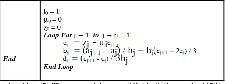
equations. This produces a natural cubic spline and leads to a simple tridiagonal system which can be solved easily to give the coefficients of the polynomials [20].Algorithm (2) describes the Cubic Spline method in sequential steps. For instance, consider one dimensional spline for a set of

points given as , then the th piece of the spline be

represented as:

… (6)

Where t is a parameter t [0,1] and i=1,2,…n-1 Taking the derivative of in each interval then gives … (7)

… (8)

… (9)

Solving (2.7)-(2.9) for and , then gives … (10)

… (11)

v … (12)

… (13)

Now require that the second derivatives also match at the points, so … (14)

… (15)

… (16)

… (17)

for interior points, as well as that the endpoints satisfy … (18)

… (19)

This gives a total of equations for the unknowns. To obtain two more conditions, require that the second derivatives at the endpoints be zero, so … (20)

… (21)

= … (22)

If the curve is instead closed, the system becomes

= … (23)

Input

( , ) , ( , ) … ,( , ) \\ Define a set of n control points.

Output ( , ) for j=0, 1,…, n-1

Procedure: Loop For to = - End Loop

Loop For to

(a

- a

) -

(a

- a

)

Ɩ

= 1

µ

= 0

ɀ

= 0

Loop For to

Ɩ

= 2(x

– x

) – h

-

µ

µ

= h

/ Ɩ

ɀ

= (

h

_-

ɀ

) / Ɩ

End

Ɩ0 = 1

µ0 = 0 ɀ0 = 0

Loop For to

= ɀ

-

µ

= (a

– a

) / h

–

h

(

= (

/ 3h

End Loop

Algorithm (2) The sequential steps of Cubic Spline method [20].

5.3 Path Deflection Determination

The intended route is defined by some of reference points which should predefined before the airplane flight mission is started. One segment of the intended route is a set of straight lines each one connecting two adjacent reference points. The instantaneous intended position of the airplane is defined by any point lies on the intended route segment, while the actual position collected by the sensor.

Figure (8-a) shows the intended route as the shortest distance between the two given way (reference) points (x1,y1) and (x2,y2). If there is a deflection in the

route of the airplane, then the instantaneous position of the airplane on the actual route (xAct,yAct) will be projected on the intended route (xInt,yInt). The

selected model aims at computing the corresponding position in the intended route depending on the known data of both the two way (reference) points and

the current actual position of the airplane. Figure (8-b) shows the distancePos,

which represents the deflection of the actual position from the intended one, it is extended perpendicularly on the intended route.

Figure (8) positioning deflection.

By using the trigonometry, connecting the actual position with the start and end way (reference) points of the route segment; it yields four line segments

m1, m2, d1, and d2. The intended route segment could be described

1 1 1 2 1 2 y y x x y y x x Int Int      … (24)

by using Pythagoras theorem for the two triangles, one can find :

2 2 2 2 2 1 2

1 m d m

d    … (25)

where 2

2 2 2

2

1 (x xAct) (y yAct)

d     … (26)

2

2 2 2 2

1 (x xInt) (y yInt)

m    

… (27) 2 1 2 1 2

2 (x x) (y y)

d  _Act  _Act … (28)

2

1 2

1 2

2 (x x ) (y y )

m  _Int  _Int  … (29)

Now, the deflection in the position Pos of the airplane can be calculated as of

the distance connecting two points (actual and intended) as follows

2 2

) (

)

(x_p x_C y_P y_C Pos   

 … (30)

These deflections can be corrected by exporting correction commands (Ci)

to the control tools to change the status of the airplane by an amount is

proportional to the deflection in the flight parameter (F). The corrected state of

the control parameters for each correction duration ( t ) can be newly

formulated by taking into consideration the accumulated effect of the previous and current correction command as follows:

      n t t F k Q C 0 )

( … (31)

where, n is the number of correction intervals, k is constant related to the

controlling response (normal response is found when k=1), t is the time slot of

each correction interval, and Q is other terms may be added to the command

model. Accordingly, the corrections in the navigation status of airplane are

depending on adding the negative amount of restricted deflection of Pos .

Thus,F may be Pos, Z , or even Speed ; each issued a specific command

forwarded into its corresponding driving tool of the airplane.

6. Results and Discussion

When using equation (30) on the points listed in Table (2) to estimate the

amount of positioning deflection (Pos) for both adopted path planning methods:

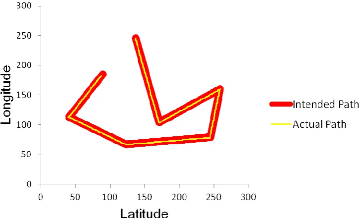
DDA and CS. The resulted deflection that is determined as the difference between the planned path and actual path is shown in Figure (10) when using the DDA method for path planning, while Figure (11) shows the deflection of the actual flight path when using the CS method for path planning.

Figure (9) Planned path of the flight test of proposed control method.

Figure (11) Flight path deflection when using CS for path planning method.

The related deflections of the actual flight deflection, in which the percent of the actual path deflection using DDA method is about 2.2%, whereas the percent of the actual path deflection using CS method is about 0.4%. This percent is determined by computing the number of points in the actual path that identify the position of the planned path divided by the total number of points in the planned path.

Results analysis of both actual and planned paths showed that CS method produces planned path is almost identifying the intended one, and this method produces gradual head changes of airplane without leading to suddenly accidents. Therefore, the results prove that the CS method is very suitable for planning the path of flight due to less path deflection is found and also slow influence to the change occurs in the head of the airplane at turns.

7. Conclusion

References

1. Dorf, R.C. and R.H. Bishop, Modern control systems. 2011: Pearson.

2. DiStefano, J.J., A.J. Stubberud, and I.J. Williams, Schaum's outline of feedback and control systems. 1997: McGraw-Hill Professional.

3. Åström, K.J. and T. Hägglund, PID controllers: theory, design, and tuning. Vol. 2. 1995: Instrument society of America Research Triangle Park, NC.

4. Altaei, M.S.M., Dynamic Navigator For UAV, Physics, Editor. 2007: Al-Nahrain University.

5. Serway, R. and J. Jewett, Principles of physics: a calculus-based text. Vol. 1. 2012: Nelson Education.

6. Anderson Jr, J.D., Fundamentals of aerodynamics. 2010: Tata McGraw-Hill Education.

7. Reviews, C., Calculus, One and Several Variables. 2016: Cram101.

8. Shevell, R.S. and R.S. Shevell, Fundamentals of flight. Vol. 2. 1989: Prentice Hall Englewood Cliffs, NJ.

9. Bolstad, P., GIS Fundamentals: A First Text on Geographic Information Systems. 2005: Eider Press.

10. Staff, O., Waypoint Definition in English. 2017.

11. Greenhalgh, R., et al., Endovascular aneurysm repair and outcome in patients unfit for open repair of abdominal aortic aneurysm (EVAR trial 2): randomised controlled trial. 2005. 365(9478): p. 2187-2192.

12. Babaei, A., M.J.A.E. Mortazavi, and A. Technology, Fast trajectory planning based on in-flight waypoints for unmanned aerial vehicles. 2010. 82(2): p. 107-115.

13. Gray, J., B.J.S. Rumpe, and S. Modeling, Models in simulation. 2016. 15(3): p. 605-607.

14. Jun, M. and R. D’Andrea, Path planning for unmanned aerial vehicles in uncertain and adversarial environments, in Cooperative control: models, applications and algorithms. 2003, Springer. p. 95-110.

15. Haque, S.R., R. Kormokar, and A.U. Zaman. Drone ground control station with enhanced safety features. in Convergence in Technology (I2CT), 2017 2nd International Conference for. 2017. IEEE.

16. Monwar, M., O. Semiari, and W.J.a.p.a. Saad, Optimized Path Planning for Inspection by Unmanned Aerial Vehicles Swarm with Energy Constraints. 2018. 17. Shi, Z. and W.K.J.a.p.a. Ng, A Collision-Free Path Planning Algorithm for

Unmanned Aerial Vehicle Delivery. 2018.

18. Tutika, C.S., et al., Cubic Spline Interpolation Segmenting over Conventional Segmentation Procedures: Application and Advantages. 2018.

19. Angel, E., What is Computer Graphics? 2013.