Vladislav Kovtun1, Jan Pelzl2, and Alexandr Kuznetsov3
1 Telecommunication and Information Security Research Lab, Kharkiv Air Force University, str. Sumska 77/79, Kharkiv, Ukraine
2 Escrypt, Lise-Meitner Allee 4 44803 Bochum, Germany
3 Telecommunication and Information Security Research Lab, Kharkiv Air Force University, str. Sumska 77/79, Kharkiv, Ukraine
Abstract. This paper describes the system parameters and software implementation of a HECDSA cryptosystem based on genus-2 hyperelliptic curves over prime fields. We show how to reduce the computational complexity for special cases and compare the given cryptosystem with the well-known ECDSA cryptosystem based on elliptic curves.
Keywords: Hyperelliptic curve, divisor addition, efficient implementation, HECDSA.
Introduction
With the recent boost of information technology in modern society, the problem of information security becomes of special urgency. The most difficult task is to provide a secure handling and storage of critical and confidential data for government and private companies, banks and other systems. A solution to this problem is to implement systems which provide information confidentiality, integrity, authenticity and accessibility by means of cryptographic software and cryptographic hardware.
In recent decades, elliptic curve cryptosystems (ECC) have been widely exploited which can be seen by recent standardization efforts [1, 2]. However, this is not the last frontier of the research focused on algebraic curve application in cryptography. The authors of [3] have shown that elliptic curves have a worthy alternative, namely hyperelliptic curves (HEC) [4]. The standardization of ECC gave rise to intensive investigation of HEC properties. The biggest advantage of HEC over EC lies in its richer source of finite Abelian groups and the use of smaller finite fields.
Till now, however, most research has been done on several theoretical aspects of hyperelliptic curve cryptosystems (HECC), including many improvements of the underlying arithmetic on HEC. On the implementational side, improvements for specific processors and hardware platforms have been analyzed. With this contribution, we are providing a very important step towards the practical implementation of HECC by showing how to build an efficient HECDSA implementation and provide cryptographically suitable curves. Unfortunately, published results on practical implementation of HECC are rare [5, 6]. This paper is intended to provide very practical facts for the implementation of an HECDSA system with all its necessary details. There are a lot of modern articles dealing with HECC; but they describe no validated system parameters for the efficient implementation of a workable cryptosystem.
The lack of publications dedicated to exactly this topic gave us the motivation to carefully summarize all results for efficient HECC implementation, and compare HECC (HECDSA) with the existent ECC (ECDSA).
Finite Field Arithmetic
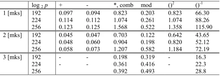
Arithmetic in the Jacobian is based on the arithmetic in a polynomial function ring over a finite field, i.e., all the transformations in the Jacobian consist of manipulation over finite field elements. In accordance with the introductory part, this paper does not focus on the finite field arithmetic and its efficient implementation. The implementation was based on results published in [7, 8, 24]. The resulting timings of arithmetic in the finite field is comparable to [8] but is worse in 3-4 times than [24] and is summarized in Table 1.
Table 1. Experimental valuations of prime base fields arithmetics timings
log 2p + - *, comb mod ()2 ()-1
1 [mks] 192 0.097 0.094 0.823 0.203 0.823 66.30
224 0.114 0.112 1.074 0.261 1.074 88.26 256 0.123 0.125 1.568 0.522 1.358 115.90
2 [mks] 192 0.045 0.047 0.703 0.122 0.642 43.65
224 0.048 0.060 0.904 0.198 0.820 52.12 256 0.058 0.073 1.207 0.582 1.184 72.19
3 [mks] 192 - - 0.198 0.319 - 16.3
224 - - 0.361 0.416 - 22.3
In Table 2, information about the platform, set-up and compiler can be found.
Table 2. General set-up of the implementation of the finite field arithmetic
Col # Source CPU Implementation features
1 [8] Intel, Pentium II 400 MHz MS VC++ 6.0 (with asm) 2 authors AMD, Athlon XP 2500+ MHz MS VC++ 2005 (w/o asm) 3 [24] AMD, Athlon 1 Ghz gcc C compiler v.2.95.3, v3.1.1
All finite fields in Table 1 are taken from the recommended elliptic curve list [9]. Table 3 provides base fields for HEC. In Table 4, fields with Jacobian order for HECDSA are given.
Table 3. Experimental results of prime base field arithmetic [mks]
Field name and description + *, comb mod ()2 ()-1
BF1, GF(p80): p1=1208925819614629175095961 0.020 0.921 0.782 0.90 0.94 BF2, GF(p88): p2=1208925819614629174708801 0.020 0.922 0.797 0.90 11.0 BF3, GF(p81): p3=2417851639229258349419161 0.020 0.922 0.797 0.9 10.5 BF4, GF(p81): p4=4835703278458516698822641 0.020 0.922 0.781 0.9 10.5 BF5, GF(p161): p5=292300327466180583640736
9665432566039311865180529
0.032 2.57 2.15 2.5 34.4
BF6, GF(p84): p6=5000000000000000008503491 0.020 0.922 0.781 0.9 11.0 As we can see from Table 3, most of the time spent for multiplication and squaring is consumed by the modular reduction. This is related to the classical modular reduction algorithm which we applied in this case. For a speed-up, the classical algorithm will be replaced with special algorithms for Mersenne and pseudo-Mersenne primes that allow for a very efficient reduction in these fields.
Table 4. Experimental results for prime order fields arithmetic [mks]
Field name and description + *, comb mod ()2 ()-1
OF1, GF(p159): p7=730750818666480869498570
026461293846666412451841 0.032 1.92 1.62 1.6 26.6
OF2, GF(p171): p8=0x00000f9e 0x508f99f1 0x9fb43a71 0x1cd119ae 0xe6bd912d 0x2bc254b9
0.031 2.563 2.14 2.53 34.3
OF3, GF(p161): p9=923003274662325095624062
806971100286403110276481 0.031 2.578 2.20 2.56 32.9
OF4, GF(p162): p10=11692013098643346868341 581279699385077839029966801
0.031 2.562 2.15 2.54 32.9
OF5, GF(p320): p11=4271974071841820164790 042159200669057836414062331724137933565 193825968686576267080087081984838097
0.047 7.40 6.14 7.35 107.6
OF6, GF(p164): p12=24999999999994130438600
Elliptic Curves
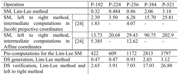
As experimental results of operations timings in the group of points on an elliptic curve, we used curves as listed in [9]. For the implementation, we used Jacobi projective coordinates [2]. In Table 5, SM – Scalar multiplication, DS – Digital signature.
Table 5. Experimental results of the arithmetic on elliptic curves and results from [24], [ms]
Operation P-192 P-224 P-256 P-384 P-521
SM, Lim-Lee method 0.32 0.484 0.86 2.06 3.18
SM, left to right method, intermediate computations in Jacobi projective coordinates
2.39 3.50 6.28 15.70 25.81
[24] 1.83 - 4.07 - -
SM, left to right method, intermediate computations in Affine coordinates
13.73 20.68 29.43 90.75 202.9
[24] 5.385 - 12.62 - -
Pre-computations for the Lim-Lee SM 422 609 1172 2813 3797 DS generation, Lim-Lee method 0.47 0.47 0.93 2.03 3.12 DS verification, Lim-Lee method and
left to right method
2.65 3.91 7.03 17.03 26.88
The results are to be in accordance with the results published in [7, 8]. Note, the results from [24] in Table 5 are given for reference. These are based on the high performance finite field arithmetic library and indicate how finite field arithmetic could affect the ECC and HECC’s performance. This allows us to use these for a comparison to the HECC transformation.
In the next section, we will describe the HECC transformations.
Hyperelliptic Curves
We analyze the transformations in the Jacobian of genus 2 HEC in affine coordinates; this allows us to select a curve type and a transformation which provides for the least computational complexity.
Table 6. Complexity of arithmetic in the Jacobian of genus 2 HEC according to Harley’s method (expressed in field operations inversion, squaring, and multiplication)
Conditions Addition Doubling I S M I S M
h(x) = 0 [12] 2 27 2 30
h2= 1 [13] 2 3 24 2 6 26
h(x) = 0 [16] 2 25 2 27
h(x) = 0, f4 = 0 [17] 1 26 1 27
h(x) = 0 [18] 1 25 1 29
For the software implementation of the transformations in the Jacobian, we used Harley’s [12] method and Lange’s [13] method for HEC over prime fields. All algorithms are given in pseudo code. A detailed functional description is commented.
Divisor Addition
In the software implementation, we made suppositions that made no contradiction to [12, 13]:
• curve parameters h2, h1, h0 from {0, 1}; • curve parameters f4, f3, f2, f1, f0∈GF(p), f5= 1.
The add divisor addition algorithm, by Harley’s method and Lange’s method has a
complex hierarchical structure. In the nodes of this structure, there are algorithms used for addition in special cases. Such architecture provides for comfortable debugging and further support. A detailed description of transformation in Jacobian can be found in [12, 13]. During paper writing, authors have found a number of mistakes in formulae deduction and their continued and careless re-publication from paper to paper dedicated to Jacobian arithmetic. Below, in represented algorithms, there are used only both theoretically and practically proven (validated) algorithms and expressions.
In the case of divisor addition, we considered several cases: the first case occurs when the first divisor has weight 2 (addw2wN algorithm). The second case occurs
when the first divisor has weight 1 (addw1wN algorithm), else - the first divisor is
copied.
Algorithm add. Divisor addition. Input: divisors d1 and d2 Output: divisor res
Algorithms addw2wN. Divisor addition with
first divisor weight equal 2.
Input: divisors d1 and d2, where weight(d1) = 2 Output: divisor res
1. if(weight(d1) = 2) then res = addw2wN(d1, d2) 2. else if(weight(d1) = 1) then
res = addw1wN(d1, d2) 3. else res = d2
return (res)
1. if(weight(d2) = 2) then res = addw2w2(d1, d2) 2. else if (weight(d2) =1) then
res = addw1w2(d2, d1) 3. else res = d1
return (res)
The algorithm for weight 2 divisor addition is addw2w2. This algorithm is called
most frequently. In different cases for the addition, the addw2wN algorithm considers
the second divisor of weight 2, 1 or 0.
We will consider the case of both divisors having weight 2, which is the most frequent case.
Algorithm addw2w2.Addition weight 2 divisors.
Input: divisors d1 and d2, where weight(d1) = weight(d2) = 2. ad1, ad2, ad3, ad4,
ad5 – temporary divisors.
Output: divisor res
1.1.1. res = dualw2(d1)
return (res)
1.2. if (d1.v0 = -d2.v0) and (d1.v1 = -d2.v1) then
1.2.1 res = O
return (res)
1.3. else
1.3.1. ad1.u0 = (d2.v0 - d1.v0) * (d2.v1 - d1.v1)-1 1.3.2. ad1.u1 = 1; ad1.u2 = 0
1.3.3. ad1.v0 = d1.v0 - d1.u0 * d1.v1; ad1.v1 = 0
1.3.4. res =dualw1rw2(ad1)
return (res)
2. else
2.1. z1 = d1.u1 - d2.u1 2.2. z2 = d2.u0 - d1.u0 2.3. z3 = d1.u1 * z1 + z2 2.5. r = z2 * z3 + z1^2 * d1.u0 2.6. if(r <> 0) then
2.6.1. res = addw2w2_i(d1, d2)
return (res)
2.7. else
2.7.1. xP1 = (d1.u0 - d2.u0) * (d1.u1 - d2.u1)-1 2.7.2. yP1 = xP1 * d1.v1 + d1.v0
2.7.3. z2 = xP1 * d2.v1 + d2.v0
2.7.4. ad1.u2 = 0; ad1.u1 = 1; ad1.u0 = -xP1 2.7.5. ad1.v1 = 0; ad1.v0 = yP1
2.7.6. ad3.u2 = 0; ad3.u1 = 1; ad3.u0 = d1.u1 - xP1 2.7.7. ad3.v1 = 0; ad3.v0 = d1.v0 - ad3.u0 * d1.v1 2.7.8. ad5.u2 = 0; ad5.u1 = 1; ad5.u0 = d2.u1 - xP1 2.7.9. ad5.v1 = 0; ad5.v0 = d1.v0 - ad5.u0 * d1.v1 2.7.10. if(yP1 = z2) then
2.7.10.1. ad2 = dualw1rw2(ad1) 2.7.10.2. ad4 = addw1w2(ad3, ad2)
2.7.10.3. res = addw1w2(ad4, ad5)
2.7.11. else res = addw1w1(ad3, ad5) return (res)
We will consider the case of the first divisor having weight 1. Further branching is done as per second divisor weight. We will now consider the case of the first divisor having weight 1 and the second divisor having weight 2.
Algorithm addw1wN. Addition weight 1
divisor and divisor with unknown weight
Input: divisors d1 and d2, where
weight(d1) = 1
Output: divisor res
Algorithm addw1w2. Addition weight 1
and weight 2 divisors
Input: Divisors d1 and d2, where
weight(d1) = 1, weight(d2) = 2
Output: divisor res
1. if (weight(d2) = 2) then res = addw1w2(d1, d2,) 2. else if (weight(d2) = 1) then
res =addw1w1(d1, d2)
1. r = d2.u0 – (d2.u1 - d1.u0) * d1.u0 2. if(r = 0) then
3. else res = d1;
return (res) return (res)res = addw1w2_i(d1, d2)
Now, the most common case is considered when adding divisors with weight 1 and 2. In this case the second divisor support has either point P1 or point -P1 of the first divisor support.
Algorithms addw1w2Cmn. Addition weight 1 and weight 2 divisors in common
case.
Input: divisors d1 and d2, where weight(d1) = 1 and weight(d2) = 2 Output: divisor res
1. r = d2.u0 – (d2.u1 - d1.u0) * d1.u0 2. if (r <> 0) then
2.1. res = addw1w2_i(d1, d2)
return (res)
3. if ((d2.v0 - d1.u0 * d2.v1) = d1.v0) then
3.1. res.u2 = 0; res.u1 = 1; res.u0 = d2.u1 - d1.u0 3.2. res.v0 = d2.v0 - res.u0 * d2.v1; res.v1 = 0 4. else
4.1. if (d2.u1 = 2 * d1.u0) then
4.1.1. ad2 = dualw2_i(d2)
4.1.2. ad1 = -d1
4.1.3. res = addw1w2(ad1, ad2)
4.2. else
4.2.1. ad1 = dualw1rw2(d1)
4.2.2. ad2.u2 = 0; ad2.u1 = 1; ad2.u0 = d2.u1 - d1.u0 4.2.3. ad2.v1 = 0; ad2.v0 = d2.v0 – (ad2.u0 * d2.v1)
4.2.4. res = addw1w2_i(ad2, ad1)
return (res)
We consider the case of a divisor addition having weight 1 in algorithm addw1w1
while we consider algorithm addw1w2_i of divisor addition with weight 1 and 2 in
the most frequent case.
We consider the addw2w2_i algorithm of divisor addition having weight 2 in the
most frequent case [13].
Algorithm addw1w1. Weight 1
divisor addition
Input: weight 1 divisors d1 and d2 Output: res
Addition addw1w2_i. Weight 1 divisor
and weight 2 divisor addition in most frequent case
Input: weight 1 divisor d1 and weight 2
divisor d2
Output: res
1. if (d1.u0 = d2.u0) then
1.1. if(d1.v0 = d2.v0) then
res = dualw1rw2(d1)
1.3. if(d1.v0 = -d2.v0) res = O 2. else
1. r = d2.u0 - (d2.u1 - d1.u0) * d1.u0 2. inv = (r)-1
2.1. top = (d1.u0 - d2.u0)-1 2.2. res.v1 = d2.v0 - d1.v0 2.3. res.v1 = res.v1 * top 2.4. top1 = d2.v0 * d1.u0 2.5. top2 = d1.v0 * d2.u0 2.6. res.v0 = top1 - top2 2.7. res.v0 = res.v0 * top 2.8. res.u2 = 1;
2.9. res.u1 = -(d1.u0 + d2.u0) 2.10. res.u0 = d1.u0 * d2.u0 return (res)
6. k1 = curve.f3 - k2 * d2.u1 - d2.u0 7. res.u2 = 1
8. res.u1 = (k2 - s0^2) - d1.u0 9. k2 = res.u1 * d1.u0
10. res.u0 = k1 – (2 * d2.v1 + l1) * s0- k2 11. top = s0 * res.u1
12. res.v1 = top – (l1 + d2.v1) 13. res.v0 = s0 * res.u0 – (l0 - d2.v0) return (res)
Algorithm addw2w2_i. Weight 2 divisor addition in most frequent case Input: Weight 2 divisors d1 and d2
Output: res
1. z1 = d1.u1 - d2.u1 2. z2 = d2.u0 - d1.u0 3. z3 = d1.u1 * z1 + z2 4. r = z2 * z3 + z1^2 * d1.u0 5. inv1 = z1; inv0 = z3 6. w1 = d1.v0 - d2.v0 7. w2 = d1.v1 - d2.v1
8. w3 = inv0 * w1; w4 = inv1 * w2 9. s1s = inv1 + inv0
10. w1 = w1 + w2
11. s1s= s1s * w1 - w3 - w4- w4 * d1.u1 12. s0s = w3 - w4 * d1.u0
13. if(s1s = 0) then
13.1. s0 = s0s * (r)-1
13.2. res.u0 = curve.f4 - d2.u1 13.3. res.u0 = res.u0 - d1.u1 13.4. res.u0 = res.u0 - s0^2 13.5 res.u1 = 1; res.u2 = 0 13.6. w1=(d2.u1 + res.u0) * s0 13.7. w1 = w1 + d2.v1 13.11. w2 = s0 + d2.v0 13.12. res.v0 = res.u0 * w1
Continued in the next column
continuation
13.13. res.v0 = res.v0 - w2 13.14. res.v1 = 0
return (res)
14. w1 = (r * s1s)-1; w2 = w1 * r 15. w3= s1s^2 * w1; w4 = r * w2 16. w5 = w4^2; s0ss = s0s * w2 17. l2s = s0ss + d2.u1
18. l1s = s0ss * d2.u1 + d2.u0 19. l0s = s0ss * d2.u0 20. inv0 = s0ss - d1.u1
21. res.u0=(l2s- d1.u1) * inv0 - d1.u0+ l1s 22. res.u0 = res.u0 + 2 * d2.v1 * w4 23. top = (d1.u1 + d2.u1 - curve.f4) * w5 24. res.u0 = res.u0 + top
25. res.u1 = (s0ss + l2s) - d1.u1 - w5 26. res.u2 = 1
27. w1 = l2s - res.u1
28. w2 = res.u1 * w1 + res.u0 - l1s 29. res.v1 = w3 * w2 - d2.v1 30. w4 = res.u0 * w1 - l0s 31. res.v0 = w3 * w4 - d2.v0 return (res)
Furthermore, we will describe a dual divisor doubling algorithm. In this algorithm,
the branching is depending on the weight of the doubled divisor. Algorithm dualw1 is
called when a divisor with weight 1 is doubled.
Algorithm dual. General case of divisor
doubling
Input: divisor d Output: divisor res
Algorithm dualw1. Weight 2 divisor
doubling.
1. if (weight(d) = 2) then
res = dualw2(d)
2. else if (weight(d) = 1) then
res = dualw1(d)
3. else res = O return (res)
1. if (d.v0 = 0) then
res = O
2. else
res = dualw1rw2(d)
return (res)
Algorithm dualw1rw2. Weight 1 divisor
doubling and resulting divisor has weight 2
Input: weight 1 divisor d Output: weight 2 divisor res
Algorithm dualw2. Weight 2 divisor
doubling in general case
Input: weight 2 divisor d Output: weight 2 divisor res
1. u10 = d.u0
2. res.u2 = 1; res.u1 = 2 * u10 3. res.u0 = u10^2
4. ft0 = 3 * curve.f3 - 4 * curve.f4 * u10 5. ft0 = ft0 + 5 * res.u0
6. ft0 = ft0 * res.u0
7. ft0 = ft0 - 2 * curve.f2 * u10 + curve.f1 8. res.v1 = ft0 * (2 * d.v0)-1
9. res.v0 = d.v0 + res.v1 * u10 return (res)
1. if(d.v0 =0) and (d.v1 = 0) then
res = O
return (res)
2. vt1 = 2 * d.v1; vt0 = 2* d.v0 3. w0 = d.v1^2; w1 = d.u1^2 4. w2 = vt1^2; w3 = d.u1 * vt1 5. r = d.u0 * w2 + (vt0 - w3) * vt0 6. if(r = 0) then
6.1. xP2=d.v1 * (d.v0)-1- d.u1 6.2. yP2 = xP2 * d.v1 + d.v0 6.3. ad1.u0 = -xP2
6.4. ad1.u1 = 1; ad1.u2 = 0 6.5. ad1.v0 = yP2; ad1.v1 = 0 6.6. res = dualw1rw2(ad1) 7. else res = dualw2_i(d)
return (res)
Algorithm dualw2 is called when a divisor with weight 2 is doubled. The dualw1rw2 algorithm is worth for a separate consideration since it doubles divisors
with weight 1 and produces the resulting divisor with weight 2 [12].
Let us describe algorithm dualw2_i for doubling weight 2 divisors which is the
most frequent case [13].
Algorithm dualw2_i. Weight 2 divisor doubling in most frequent case. Input: weight 2 divisor d
Output: divisor res
1. vt1 = 2 * d.v1; vt0 = 2 * d.v0 2. w0 = d.v1^2; w1 = d.u1^2 3. w2 = vt1^2; w3= d.u1 * vt1 4. inv0 = vt0 - w3; inv1 = -vt1 5. r = d.u0 * w2 + inv0 * vt0
continuation
14.5. res.v0 = res.u0 * w1 - w2 14.6. res.v1 = 0
14.7. res.u1 = 1; res.u2 = 0
6. w3 = w1 + curve.f3 7. w4 = 2 * d.u0 8. top = curve.f4 * d.u1
9. k1 = 2 * (w1 – top) + w3 – w4
10. k0 = (2* w4 + top – w3) * d.u1 + curve.f2 - w0 - 2 * curve.f4 * d.u0 11. w0 = k0 * inv0; w1 = k1 * inv1 12. s1s = (k1 + k0) * (inv1 + inv0) – w0 - (d.u1 + 1) * w1
13. s0s = w0 - w1 * d.u0 14. if (s1s = 0) then
14.1. s0 = s0s * (r)-1 14.2 w2 = s0 * d.u0 + d.v0
14.3.res.u0=curv.f4-s0^2-2*d.u1 14.4. w1=s0*(d.u1-res.u0)+ d.v1 continued in the next column
15. w1 = (r * s1s)-1; w2 = r * w1 16. w3 = s1s^2 * w1; w4 = r * w2 17.; w5 = w4^2; s0ss = s0s * w2 18. l2s = d.u1 + s0ss
19. l1s = d.u1 * s0ss + d.u0 20. l0s = d.u0 * s0ss
21. res.u0=s0ss^2+(2*d.u1-curve.f4)* w5 22. res.u0 = res.u0 + 2 * d.v1 * w4 23. res.u1 = 2 * s0ss - w5; res.u2 = 1 24. w1 = l2s - res.u1
25. w2 = res.u1 * w1 + res.u0 - l1s 26. res.v1 = w2 - w3 - d.v1 27. w4 = res.u0 * w1 - l0s 28. res.v0 = w4 * w3 - d.v0 return (res)
Complexity Analysis
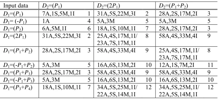
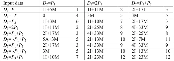
In this section, we will provide an analysis of the complexity of the transformations of divisor addition considering different input data given in Table 7. For the sake of a compact representation, in Table 7 the input divisors were given without point at infinity P∞. As we stated above, this work is based on the transformation described at [12, 13], however we have made several improvements in the cases other than the most frequent cases in comparison to [13, 16].
Table 7. Complexity of divisor addition algorithms in relation to input divisors
Input data D2=(P1) D2=(2P1) D2=(P1+P2)
D1=(P1) 7A,1S,5M,1I 1 31A,5S,22M,3I 2 28A,2S,17M,2I 3
D1= (-P1) 1A 4 5A,3M 5 5A,3M 5
D1=(P2) 6A,5M,1I 6 18A,1S,10M,1I 7 28A,2S,17M,2I 3
D1=(2P1) 31A,5S,22M,3I 2 25A,4S,17M,1I/
23A,7S,17M,1I 8 58A,4S,33M,4I 9
D1=(P1+P2) 28A,2S,17M,2I 3 58A,4S,33M,4I 9 25A,4S,17M,1I/ 23A,7S,17M,1I
8
D1=(-P1+P2) 5A,3M 5 16A,6S,13M,2I 10 12A,1S,7M,2I 11
D1=(P1+P3) 28A,2S,17M,2I 3 58A,4S,33M,4I 9 58A,4S,33M,4I 9
D1=(-P1+P3) 5A,3M 5 16A,6S,13M,2I 10 16A,6S,13M,2I 10
D1=(P3+P4) 18A,1S,10M,1I 7 34A,5S,25M,1I/
The second term after the slash sign provides the complexity of weight 2 divisor addition algorithms which are given for the case of the resulting divisor of weight 1.
We will now compare the results given in Table 7 and the results given in Table 8 obtained from [16]. (Formulas from [13] are more efficient than [16], but, unfortunately, [13] does not contain summarized results as in Tables 7, 8.) With these tables, we get a more exact picture of complexity of the algorithms than before. Furthermore, these exact values are characterized by the decreased complexity for the most frequent cases. Authors propose optimized execution ways for the general case divisor addition which allows for an increase in Jacobian arithmetic performance.
Table 8. Divisor addition algorithms complexity in relation to input divisors obtained from [16]
Input data D2=P1 D2=2P1 D2=P1+P2
D1=P1 1I+5M 1 1I+11M 2 2I+17I 3
D1= -P1 0 4 3M 5 3M 5
D1=P2 1I+3M 6 1I+10M 7 2I+17M 3
D1=2P1 1I+11M 2 2I+25M 8 4I+33M 9
D1=P1+P2 2I+17M 3 4I+33M 9 2I+25M 8
D1= -P1+P2 5A+3M 5 2I+13M 10 2I+7M 11
D1=P1+P3 2I+17M 3 4I+33M 9 4I+33M 9
D1= -P1+P3 3M 5 2I+13M 10 2I+13M 10
D1=P3+P4 1I+10M 7 2I+23M 12 2I+23M 12
Experimental Results
To be able to provide practical results, we executed the experimental evaluation of Jacobian arithmetic and direct cryptographic transformations. In Table 9, we provide the respective parameters. All the experiments were executed in accordance to the conditions described in Table 1, column 2.
Table 9. List of parameters that have been evaluated in the experimental timing evaluation while operations were executed in the Jacobian of genus 2 HEC in affine representation
# Operation
1 Weight 2 divisor addition, D1=(P1+P2), D2=(P3+P4), different points in support 2 Weight 1 divisor addition, D1=(P1), D2=(P2), different points in divisors support 3 Weight 2 divisor doubling, D1=(P1+P2), different points in divisors support 4 Weight 1 divisor doubling, D1=(P1), different points in divisors support 5 Pre-computations for Lim-Lee SM of weight 2 divisor, D1=(P1+P2) 6 Weight 2 divisor SM, D1=(P1+P2), Lim-Lee method
7 Weight 2 divisor SM, D1=(P1+P2), left to right (l-to-r) method 8 Pre-computations for Lim-Lee SM of weight 1 divisor, D1=(P1) 9 Weight 1 divisor SM, D1=(P1), Lim-Lee method
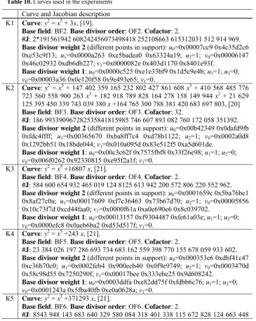
The performance estimation for HECDSA was executed for curves from different sources. For each curve, the prime group order and base divisors of different weight are specified. Table 10 could be used for building a workable cryptosystem. It summarizes all required system parameters from the latest publications dedicated to system parameters generation. These base divisors are generated using authors’ Jacobian arithmetic library.
Table 10. Curves used in the experiments
Curve and Jacobian description K1 Curve: y2 = x5 + 3x, [19].
Base field: BF2. Base divisor order: OF2. Cofactor: 2.
#J: 2*191561942 608242456073498418 252108663 615312031 512 914 969. Base divisor weight 2 (different points in support): u0=0x00007cc9 0x4c35d2c6 0xe53c9f13; u1=0x0000a263 0xe5badea0 0x63324a19; u2=1; v0=0x00006147 0x46c02932 0xdb6db227; v1=0x0000082e 0x403d1170 0x8401e93f.
Base divisor weight 1: u0=0x0000c525 0xe1e33bf9 0x1d5c9e4b; u1=1; u2=0;
v0=0x00003a36 0x0e120f58 0x9e493e65; v1=0.
K2 Curve: y2 = x5 + 147 402 359 165 232 802 427 861 608 x5 + 410 568 485 776
723 560 558 900 263 x3 + 182 918 789 828 164 278 158 149 944 x2 + 21 629
125 395 450 339 743 039 380 x +164 765 300 788 381 420 683 697 803, [20] Base field: BF3. Base divisor order: OF3. Cofactor: 32.
#J: 186 993390967282535841815985 746 607 893 082 760 172 058 351392. Base divisor weight 2 (different points in support): u0=0x00b42349 0x0dafd9fb 0xfdc4ffff; u1=0x00365670 0xba8ff7c4 0xd78b1122; u2=1; v0=0x0002a0d8 0x1292bb51 0x18bde044; v1=0x010a095d 0x83e512f5 0xa5d601de.
Base divisor weight 1: u0=0x00c3c62f 0x7575fbf8 0x33f26e98; u1=1; u2=0;
v0=0x006f0262 0x92330815 0xe95f2a1f; v1=0. K3 Curve: y2 = x5 +16807 x, [21].
Base field: BF4. Base divisor order: OF4. Cofactor: 2.
#J: 584 600 654 932 465 019 124 8125 613 942 200 572 806 220 552 962. Base divisor weight 2 (different points in support): u0=0x0001659c 0x5ba76be1 0x8af27c0a; u1=0x00017609 0xf7c36463 0x73b67d70; u2=1; v0=0x00005856 0x10c73f7d 0xcd44faa0; v1=0x0000f61a 0xa0e690e6 0x8c039702.
Base divisor weight 1: u0=0x00013157 0xf9304487 0xfe61a03e; u1=1; u2=0;
v0=0x0000efc8 0x0aeb6ba2 0xd53d517f; v1=0. K4 Curve: y2 = x5 +243 x, [21].
Base field: BF5. Base divisor order: OF5. Cofactor: 2.
#J: 23 384 026 197 286 693 734 683 162 559 398 770 155 678 059 933 602. Base divisor weight 2 (different points in support): u0=0x000353e6 0xdbf41c47 0xc36b70c0; u1=0x0002feb4 0x900ecb40 0x0f9e9749; u2=1; v0=0x0003470d 0x58c98d55 0x7250290f; v1=0x00017bee 0x333ebe25 0x9d608242.
Base divisor weight 1: u0=0x0003ddfa 0xe82dd75f 0xfdbb6c76; u1=1; u2=0;
v0=0x0001243a 0x5fba40fb 0xe0a0628a; v1=0.
К5 Curve: y2 = x5 +371293 x, [21].
Base field: BF6. Base divisor order: OF6. Cofactor: 2.
275 867 130 387 651 937 273 152 534 160 174 163 969 676 194.
Base divisor weight 2 (different points in support): u0=0x00000000 0x0a666ced 0x9e3224f6 0x94fdac4a 0xa1694f53 0x4e67b73a; u1=0x00000001 0xfc7689a3 0xf3f58c91 0xf7d4367f 0xf8a69ba3 0xf8ac347e; u2=1; v0=0x00000000 0x9348b4a9 0x15fbaea2 0x100be54d 0x90a91887 0x71600c09; v1=0x00000000 0x1427f768 0x2888c86a 0x5aaf4273 0xd9bf0b9e 0x336ccd43.
Base divisor weight 1: u0=0x00000001 0xf11030ad 0xfab1afdf 0xdad8b1bd 0xf716f596 0x31eea096; u1=1; u2=0; v0=0x00000000 0x186e086c 0xa0f1d327 0x6fbced02 0x1e77e117 0x412efc16; v1=0.
K6 Curve: y2 = x5+ 2682810822839355644900736x3 + 226591355295 993102902
116x2+2547674715952929717899918x+4797309959708489673059 350, [22]. Base field: BF7. Base divisor order: OF6. Cofactor: 1.
#J: 24 999 999 999 994 130 438 600 999 402 209 463 966 197 516 075 699. Base divisor weight 2 (different points in support): u0=0x0001f086 0x14077642 0x85553ac5; u1=0x0001f031 0x4761f58d 0xa0c1db51; u2=1; v0=0x0000af4b 0x71adc1da 0x67827fe6; v1=0x0000304c 0x013ba45f 0xc74e75ca.
Base divisor weight 1: u0=0x0000eae9 0xd24b61c0 0x776e2f95; u1=1; u2=0;
v0=0x0003860b 0x36744576 0xb26dd538; v1=0.
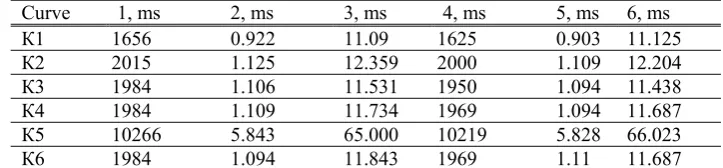
In Table 11, we provide the experimental timing estimates of group operations for the curves from Table 9 and the parameters from Table 8.
From Table 11, one can see that the time of addition and doubling for weight 1 divisors is about 2 times less than for weight 2 divisors. The time for doubling is 2 times larger than the addition time of weight 2 and weight 1 divisors.
Co-factors with large Hamming weight obviously reflect on the pre-computation time for curves K1 and K2.
Table 11. Experimental results of operations in the Jacobian of genus 2 HEC in affine representation
1 [ms] 2 [ms] 3 [ms] 4 [ms] 5 [ms] 6 [ms] 7 [ms] 8 [ms] 9 [ms] 10 [ms]
К1 0,036 0.0156 0.0469 0.0218 1656 0.86 9.65 1625 0.625 2.891
К2 0,035 0.0171 0.0484 0.0219 2015 1.062 9.844 2000 0.657 2.875
К3 0,0359 0.0156 0.0469 0.0219 1984 1.031 9.563 1950 0.73 2.891
К4 0.0375 0.0156 0.0468 0.0219 1984 1.031 9.594 1969 0.73 2.906
К5 0.103 0.0469 0.1328 0.0641 10266 5.64 55.35 10219 2.719 8.297
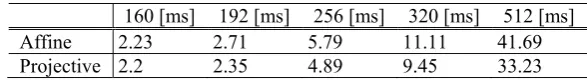
К6 0.0359 0.0172 0.0468 0.0203 1984 1.063 10.56 1969 1.11 9.57 Unlike in Table 12, let’s demonstrate the results published in [24]. Unfortunately, [24] does not describe the HECs used.
Table 12. Experimental results of SM in the Jacobian of genus 2 HEC in affine and projective representation for the specified bit length of base field [24]
160 [ms] 192 [ms] 256 [ms] 320 [ms] 512 [ms]
Affine 2.23 2.71 5.79 11.11 41.69
The time required for a scalar multiplication is essentially affected by the non-optimized finite field arithmetic and is implementation. As we can see, in Table 12, there is used a highly efficient base field arithmetic implementation [24].
The next step is the estimate of performance of an HECDSA implementation. In Table 13, we show the parameters which are of particular interest, SM – Scalar multiplication, DS – Digital signature.
Weight 1 divisors are the most interesting ones since they allow to decrease the computational complexity. This result was presented in [23]. Furthermore, we will emphasize the optimized transformation implementation based on weight 1 base divisors.
Table 13. Parameters for the timing analysis of operations in the Jacobian of genus 2 HEC in affine representation
# Operation
1 Pre-computations for the weight 2 divisor SM by Lim-Lee method, D1=(P1+P2) 2 DS generation, weight 2 base divisor, D1=(P1+P2), Lim-Lee method
3 DS verification, weight 2 base divisor, D1=(P1+P2), Lim-Lee and l-to-r methods 4 Pre-computations for the weight 1 divisor SM by Lim-Lee method, D1=(P1) 5 DS generation, weight 1 base divisor, D1=(P1), Lim-Lee method
6 DS verification, weight 1 base divisor, D1=(P1), Lim-Lee and l-to-r methods
Table 14. Experimental timings for HECDSA cryptographic transformations in the Jacobian of genus 2 HEC in affine divisor representation for curves listed in Table 9
Curve 1, ms 2, ms 3, ms 4, ms 5, ms 6, ms
К1 1656 0.922 11.09 1625 0.903 11.125
К2 2015 1.125 12.359 2000 1.109 12.204
К3 1984 1.106 11.531 1950 1.094 11.438
К4 1984 1.109 11.734 1969 1.094 11.687
К5 10266 5.843 65.000 10219 5.828 66.023
К6 1984 1.094 11.843 1969 1.11 11.687
Digital signature verification time is much influenced by operations in the field of prime group order module. In this case, specialized algorithms using pseudo-Mersenne and pseudo-Mersenne primes are not applicable.
Summary
This contribution does provide detailed information of algorithms, curves, and underlying arithmetic algorithms for the implementation of HECC in applications. With this paper, we hope to bring HECC a major step towards practical applications.
Bibliography
1. ISO/IEC FCD 15946: Information technology – Security techniques – Cryptographic techniques based on elliptic curves, Final Committee Draft. –2001.
2. IEEE P1363–2000: Standard Specifications for Public Key Cryptography. –2000. –206p. 3. Koblitz N. Hyperelliptic cryptosystems // Journal of cryptology. –1989. –No.1. –pp.139–150. 4. Menezes A.J., Wu Y., Zuccherrato R.J. An elementary introduction to hyperelliptic
curves // Technical report CORR96-19, Department of Comboinatorics and optimization, University of Waterloo, Waterloo, Ontario, 1996. In: Koblitz, N.: Algebraic aspects of cryptography, Springer-Verlag, Berlin Heidelberg New York. 1998.
5. Moreno R., Miret J.M., Sebe F. A hyperelliptic cryptosystem based on the P1363 IEEE standard // International Meeting On Coding Theory And Cryptography. IMCTC’99. -1999. –Medina.
6. N.P.Smart. On the Performance of Hyperelliptic Cryptosystems // In Advances in Cryptology – Eurocrypt’99. –LNCS 1592. –Springer. –Berlin. –pp. 165-175.
7. Hankerson D., Lopez J., Menezes A. Software implementation of elliptic curve cryptography over binary fields / In Cetin K. Koc and C. Paar editors // Workshop and embedded systems. –LNCS 1717. –Berlin: Springer–Verlag, 2000. –pp.1–24.
8. Brown M., Hankerson D., Lopez J., Menezes A. Software implementation of the NIST elliptic curves over prime fields // Research Report CORR 2000–56. Department of Combinatorics and Optimization, University of Waterloo. –Canada: Waterloo, Ontario, 2000. –21p.
9. National Institute of Standards and Technology, Recommended Elliptic Curves for Federal Government Use, Appendix to FIPS 186-2, 2000. –43p.
10. Nagao K. Improving Group Law Algorithms for Jacobians of Hyperelliptic Curves // In W. Bosma, editor, ANTS IV, LNCS 1838. –Berlin. –Springer-Verlag. –pp. 439–448.
11. Wollinger T. Software and hardware implementation of hyperelliptic curve cryptosystems. PhD dissertation: Electronics and informatics. –Worchester Polytecnic Institute. –Germany: Bochum, 2004. –218 p.
12. Harley R. Fast arithmetic on genius two curves. –2000. Available at:
http://cristal.inria.fr/harley/hyper/, adding.txt and doubling.c.
13. Lange T. Formulae for Arithmetic on Genus 2 Hyperelliptic Curves // Applicable Algebra in Engineering, Communication and Computing. -2004. LNCS vol. 15, No 5, Springer, 2004, -pp. 259-328.
14. Kovtun V. Yu., Zbitnev S. I. Arithmetic in Jacobian of genus 2 Hyperelliptic curve in projective coordinates with reduced complexity // Vostochno-Evropeyskiy zhurnal peredovikh tekhnologiy. -2004. –Vol. ½ (13). -Kharkov. –pp. 14–22.
15. Kovtun V.Yu. Transformations in Jacobian genus 2 HEC in projective coordinates over odd characteristic fields // Radiotekhnika: Vseukrainskiy mezhvedomstvenniy nauchno-tekhnicheskiy sbornik. -2006. –Vol. 144. –Karkov. -pp. 102-110. In Russian.
16. Matsuo K., Chao J., Tsujii S. Fast genius two hyperelliptic curve cryptosystem // Technical report IEICE. –ISEC2001–31. –IEICE`2001. –2001. –8p.
18. Takahashi M. Improving Harley algorithms for Jacobians of genius 2 hyperelliptic curves // In the 2002 Symposium on cryptography and information security. –SCIS`2002. Japan: IEICE, 2002. –pp. 155–160. In Japanese.
19. O’hEigeartaigh C. web-page: http://www.computing.dcu.ie/~coheigeartaigh/crypto.html
20. Weng A. Constructing hyperelliptic curves of genus 2 suitable for cryptography // Mathematics of Computation. -Vol. 72. –No.241. -2002. –pp. 435-458. 21. Furucawa E., Kawazoe M., Takahashi T. Counting Points on the Jacobian Variety of a
Hyperelliptic Curve defined by y^2 = x^5 + ax over a Prime Field // Electronic cryptology archive Citeseer. Available at: http://citeseer.ist.bsu.edu/558804.html
22. Gaudry P., Schost E. Construction of Secure Random Curves of Genus 2 over Prime Fields // Advances in Cryptology - EUROCRYPT 2004. -2004. C. Cachin and J. Camenisch, Eds., LNCS vol. 3027, Springer-Verlag, pp. 239-256.
23. Katagi M., Kitamura I., Akishita T., Takagi T. Novel Efficient Implementations of Hyperelliptic Curve Cryptosystems using Degenerate Divisors // Information Security Applications, 5th International Workshop - WISA 2004. -2004. LNCS vol. 3325, Springer 2004, -pp. 345-359
![Table 4. Experimental results for prime order fields arithmetic [mks]](https://thumb-us.123doks.com/thumbv2/123dok_us/1862566.1242065/3.595.120.478.487.654/table-experimental-results-prime-order-fields-arithmetic-mks.webp)