Wideband Radio Frequency Noiselet Waveforms for Multiresolution
Nondestructive Testing of Multilayered Structures
Tae Hee Kim and Ram M. Narayanan*
Abstract—Developed initially for military applications, radar technology is rapidly spreading to areas as diverse as natural resource monitoring, civil infrastructure assessment, and homeland security. Waveform design is a critical component to extract maximum information about the targets or features being probed. Waveforms derived from noiselets, one of the family functions of wavelets, can be advantageous in certain applications owing to their random and uncorrelated properties. In this work, radio frequency (RF) noiselet waveforms are introduced and their performance related to detection of arbitrary target interfaces using the cross-correlation method, a form of matched filtering, is assessed. The application of the RF noiselet waveform for nondestructive testing (NDT) of the multilayered dielectric structures is discussed. The application of wideband noiselet waveforms for multiresolution analysis (MRA) is demonstrated.
1. INTRODUCTION
Radio frequency (RF) noiselets are herewith defined as short duration pulsed waveforms containing high frequency random signals within the pulse envelope. In other words, they can be considered as frequency modulated random waveforms. A noiselet originates from the definition of wavelets and has desirable properties for radar applications, such as mutual orthogonality, a flat Fourier transform, and the potential for multiresolution analysis (MRA) [1]. The noiselet has the structure of a sparse representation and it is composed of random noise coefficients. While the noiselet can be thought of as a pulsed wavelet, it is perfectly uncorrelated to the signal representation of wavelets. Thus, it is conjectured that noiselets could have the potential of higher probability of signal detection and recovery from sparse data [1, 2].
In any radar application, good range resolution is desired to better resolve closely spaced targets and features. For frequency modulated waveforms employing matched filtering, the range resolution ∆Ris inversely proportional to the bandwidth B and is given by ∆R =c/2B√εr, wherec is the speed of light andεr is the dielectric constant of the medium [3]. A noise radar transmits a random signal and matched filtering is accomplished by cross-correlating the received signal with a time-delayed transmit signal replica. A noise radar system possesses low probability of interception (LPI), low probability of detection (LPD), and interference and jamming suppression, which are advantageous in RF-congested and RF-contested environments [4]. While a continuous wave (CW) wideband noise radar can achieve excellent range resolution based on the bandwidth, pulsed noise radars are preferred to eliminate problems associated with transmit-receive isolation and to reduce computational complexity [5]. By randomizing the signal from pulse to pulse, completely independent information is acquired from the target from each pulse [6].
Although ultrawideband (UWB) signals result in fine range resolution, feature information within multilayered structures can be better characterized by exploring the spatial neighborhood around the
Received 30 March 2018, Accepted 28 May 2018, Scheduled 4 June 2018
* Corresponding author: Ram M. Narayanan ([email protected]).
nominal detection range. This can be implemented by collecting UWB data, processing the returns over the entire bandwidth (best resolution) and also over fractions of the bandwidth (progressively degraded resolutions), and using the combined information to assess the features being probed. The wavelet transform (WT) utilizes multiscale basis functions provide MR capability by processing radar echoes from both small-scale natural resonances as well as large-scale scattering center information [7].
2. WAVELET BASED RADAR
Wavelets are useful in analyzing patterns and features according to scale and wavelet algorithms process data at different scales or resolutions [8]. Gross features of a pattern are seen when it is observed through a large window, while smaller features are seen when observed through a small window. They are especially suited for approximating data with sharp discontinuities. A wavelet prototype function, called an analyzing wavelet or mother wavelet, is adopted for wavelet analysis. The WT is exploited in the analysis of nonstationary signals as an alternative to the classical short-time Fourier transform (STFT). The WT uses short windows at high frequencies and long windows at low frequencies in comparison to the STFT which uses a constant window [9].
In wavelet analyses, general functions are represented in terms of simpler, fixed building blocks at different scales and positions [10]. Various constructions of wavelets, such as orthogonal, semiorthogonal, and biorthogonal wavelets, are used in MRA. MR decompositions permit the scale-invariant interpretation of an image [11]. At coarse resolution, image details correspond to the larger structures which provide the image context. As resolution is gradually enhanced, finer structures begin to emerge. The selection of a proper mother wavelet is necessary for extracting the dynamic features of patterns for multiresolution analysis [12]. Noiselets have also been shown to serve as excellent tools for MRA, based on their extremely wide bandwidths [13].
Since a wavelet is a small oscillatory wave existing over a short duration with finite energy, it has an amplitude quickly decaying to zero in both the positive and negative directions. This makes wavelets suitable in electromagnetic (EM) analyses, such as EM scattering from sharp edges [14] and radar reflections from targets containing scatterers at different scales [15].
The concept of a wavelet-based radar was first introduced in [16] wherein the transmitted radar waveform was encoded with coefficients corresponding to a WT. Reflected radar waveforms were decoded using an inverse WT to produce a high range resolution profile of the target. A software defined radar wherein a wavelet signal was generated by an arbitrary waveform generator and upconverted to RF was tested successfully [17]. Wavelet-based radar waveforms have been investigated for several applications, including adaptive radar [18], range sidelobe suppression [19], detection of moving targets [20], synthetic aperture radar [21], and simultaneous high resolution in range and velocity [22]. In sonar, reverberations have been simulated using noiselets formed by sums of randomly weighted and delayed copies of the original transmit pulse [23].
3. RF NOISELETS GENERATION AND PROCESSING
3.1. Noiselet Generation
We generate RF noiselets by passing the output of a suitable noise source through a bandpass filter, which generates the appropriate waveform over the selected time span. The bandpass filter permits the adjustment of the frequency bandwidth of the UWB signals to achieve the desired range resolution. In our simulations, the bandwidth wasset to 4 GHz, which yielded a range resolution of 3.75 cm in air and 2.37 cm in a fiber reinforced plastic (FRP) material of a typical dielectric constant value of 2.5.
function of the bandpass filter.
A random Gaussian noiselet is produced by a random number algorithm called the Mersenne twister (MT) [24]. The Mersenne twister achieves generation of very high-quality pseudorandom numbers with a long period length, and thus its output is free of long-term correlations. In addition, it passes several
Figure 1. Block diagram of bandpass filtering operation for noiselet generation from noise source (random coefficients) existing over the entire frequency band.
(a)
(b)
tests for randomness. The Gaussian noiselet can be considered as Gaussian noise since the entire random signal is based on a Gaussian distribution such that the expectation value for random numbers from the noiselet generation will converge to that of the Gaussian distribution. The coefficients of random Gaussian noiselets can be achieved using following operation
xk+n:=xk+m⊕
(
xuk|xlk+1 )
A fork= 0,1, . . . (2)
whereA is a matrix with identity and word vectors;xstands forw-bit words; xuk represents the upper (w−r) bits on xk; xk+1l represents the lower r bits on xk+1; ⊕ is the XOR operator; | is the OR operator. The coefficients using the MT approach are computed for random numbers between −1 and +1.
Similar to the random Gaussian noiselet, a random binary noiselet is also based on the random Gaussian coefficients; however, it takes only the polarity of random coefficients from the random Gaussian noiselet. For example, positive coefficients will converge to ‘+1’ compared to negative coefficients will automatically possess ‘−1’. Therefore, the random binary noiselet will fluctuate between ‘−1’ and ‘+1’.
Figure 2 shows sample noiselets created based on previous descriptions at time- and frequency-domains depicting both the amplitude and the power spectral density (PSD). Since the signal is generated randomly each time, each realization is uncorrelated to another. The Gaussian wavelet shows a flatter response within the 8–12 GHz passband with good roll-off in the stopband, while the binary noiselet has significant variations within the passband and significant bleeding in the stopband. Therefore, averaging of multiple realizations is required to maintain smooth out the responses within the passband and to ensure a smooth roll-off in the stopband.
3.2. Noiselet Processing
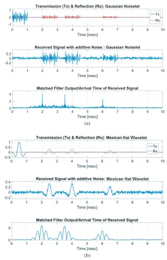
Target or feature detection is accomplished by performing the matched filter operation, i.e., cross-correlation of the transmitted waveform with the received reflected waveform. Appropriate signal attenuation and time delays are introduced in the received waveform based upon the dielectric properties of the media through which the signal passes. Also, additive uncorrelated noise signals to the received waveform to simulate realistic field situations. After the matched filtering operation is performed, the highest peak locations yield the range to the target or feature of interest.
Let xt(t) represent the transmit signal andxr(t) =axt(t−t0) represent the reflected signal from a target with a round trip time delay t0, where a is the signal attenuation factor (0 ≤ a ≤ 1). The corresponding Fourier transforms are denoted by Xt(ω) and Xr(ω), respectively. Matched filtering is performed in the frequency domain by multiplying the two Fourier transforms and then taking the inverse Fourier transform (IFT) to return to the time domain. Thus, the matched filter output Fourier transform, Xmf(ω), is given by
Xmf(ω) =Xt(ω)·Xr(ω) (3)
and its time domain representation isxmf(t) = IFT{Xmf(ω)}. The location of the peak of the matched filter response provides the range to the target.
Figure 3 shows a comparison in performance between the random Gaussian noiselet and a traditional wavelet used frequently, namely the Ricker or the Mexican hat wavelet. This wavelet is defined as the negative normalized second derivative of a Gaussian function, and is given by
x(t) = √ 2 3σπ1/4
(
1−
( t σ
)2)
e− t
2
2σ2 (4)
(a)
(b)
Figure 3. Arbitrary multiple target detection by using (a) random Gaussian noiselet, and (b) Mexican hat wavelet.
be noted that the sidelobes on the matched filter output for the Mexican hat wavelet may cause false detection or degradation of image resolution.
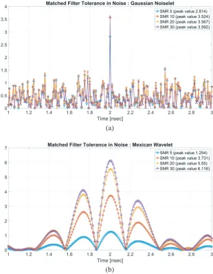
(a)
(b)
Figure 4. Performance under various SNR values for (a) random Gaussian noiselet, and (b) Mexican hat wavelet.
4. MULTILAYER SCATTERING
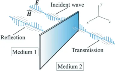
To understand the principal function of a microwave imaging system, it is important to briefly discuss how transmissions and reflections of traveling EM waves occur and propagate through various media interfaces. The thin layer shown in Fig. 5 is defined as the interface, or boundary, between medium 1 and 2. Assuming a uniform plane wave interacts with the boundary at normal incidence, it is seen that two phenomena occur — a portion of the EM wave is reflected back into medium 1, while another portion is transmitted into medium 2. Since every medium has unique material properties, transmission and reflection on each interface will provide information based on the boundary conditions.
The EM wave of Fig. 5 can be defined as a wave traveling in thez-direction. The coordinates of all figures and equations will be based on the samex-,y-, andz-direction coordinate system for consistency and simplicity of discussion. The electric fields in a transmission/reflection type EM model are given by the following expressions:
⃗
Ei = ˆyE0ie−jk1z (Incident wave) (5)
⃗
Figure 5. Uniform plane wave schematic at the interface between materials.
Figure 6. Wave propagation on interfaces for reflection data collection scheme.
⃗
Er = ˆyE0re+jk1z (Reflected wave) (7) where E0i,t,r is the corresponding amplitude of each wave, and k1,2 is the corresponding wave number, which is based on the material properties of the media. The wave number is related to the angular frequencyω, permittivity ε, and permeability µ using [25]
ki =ω√εiµi (8)
Since the uniform plane waves travel between interfaces of each media, transmission and reflection should be expressed based on the location of observation. As can be seen in Fig. 6, the sensor is placed on the left side of the sample so that the system will collect the total reflected wave from the specimen. It is to be noted that there are two boundaries: 1) air to material, and 2) material to air, which will lead to the total reflection, Γtotal, which may be obtained from
Γtotal=
E1−
E1+
= R1+R2e
−2jk1d
1 +R1R2e−2jk1d
= R1+R2e
−2jθ1
1 +R1R2e−2jθ1
(9)
whereR1 and R2 are the reflection coefficients of each interface, which are based on the relationship of the intrinsic impedance of materials with respect to the material properties.
The electrical length θi is proportional to the product of wavenumber ki and physical thickness d of the dielectric layer as can be seen from Eq. (10). In general, the reflection coefficient Ri and the intrinsic impedance Zi at the interface of the i-th and the (i+ 1)-th layer can be described as
Ri =
Zi+1−Zi
Zi+1+Zi
, Zi =
√ µi
εi
, θi =kid (10)
Expanding to the case of multilayered or multi-interface materials, it can be easily obtained using the generalized propagation matrix for thei-th layer and derived as
[ Ei+
Ei−
]
= 1
Ti
[
1 Ri
Ri 1
] [
ejθi 0
0 e−jθi ]
1
Ti+1
[
1 Ri+1
Ri+1 1
] [
E′(i+1)+ 0
]
(11)
which results in an expression similar to Eq. (9) as
Γi=
Ei−
Ei+
= Ri+Ri+1e
−2jθi
1 +RiRi+1e−2jθi
(12)
5. SYNTHETIC APERTURE RADAR (SAR) SCANNING
data from a relatively small aperture to create that of a much larger aperture [26]. Although SAR was originally introduced for airborne radar, it can be applied to alternative applications based on its synthetization scheme [27, 28]. For example, scanning a target may be achieved using railed system with an antenna attached.
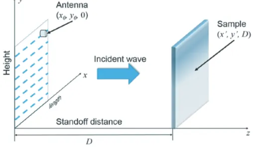
Figure 7 presents an NDT SAR imaging system for investigating multilayered FRP composites, wherex,yandzdenote the length, height and depth (or distance) of the testing specimen, respectively. As can be seen, an antenna scans over the xy-plane with a standoff distance D along the z-axis — the direction of the traveling wave. This SAR system requires a horn or lens antenna having a focused beam with a narrow beamwidth impinging on the sample at normal incidence, i.e., an incident angle of zero degrees. The antenna begins the sensing procedure at its designated point of origin and acquires data based on the sampling interval satisfying the Nyquist sampling rate to avoid aliasing effects.
Figure 7. SAR NDT scanning geometry.
5.1. SAR Imaging Algorithm Using Range Migration Algorithm
In SAR processing, there are several techniques that may be applied to optimization and calibration of image processing, such as the range-Doppler algorithm (RDA), chirp scaling algorithm (CSA), range migration algorithm (RMA), just to name a few [26, 28]. Each algorithm has strengths and weaknesses based on the waveforms and testing conditions under which it is being conducted. Since our SAR NDT scanning is performed in the near-field range, and the specimens may be considered static targets, the range migration algorithm (RMA) provides the best choice to calibrate the received data. The near-field wavefront has a parabolic curvature by nature, hence, the received raw data will reflect with the opposite curvature compared to the original wavefront, as shown in Fig. 8.
The main feature of RMA is the exploitation of the Stolt interpolation technique [29, 30] which is the calibration process used to convert the received data into a plane wave. Stolt interpolation
received time domain data should be performed before applying this calibration process. Back to RMA — the coordinate references from Fig. 7 will be used for theoretical expansion. This expansion will be based on a single point of specimen, which will form an image data matrix once the data has been gathered at each sample point. Here, the reflection coefficient can be written as R(x, y, z) and the reflected raw data will besr(x0, y0, kr), wherekr is the wavenumber based on the operating frequency. The reflected raw signal can be represented as
sr(x0, y0, kr)≈R(x, y, z)·ejkrD·e−jkrDt (13) where Dis the standoff distance between antenna and specimen, and Dt is the distance from antenna to arbitrary target point. Dtcan be expressed as
Dt=
√
(x0−x)2+ (y0−y)2+ (−D−z)2 (14) In Eq. (13), there are two exponential terms: the first term is the reference phase between the antenna and normal incident interface of specimen, while the second term represents the phase information from the arbitrary point of specimen.
Since it is already mentioned that domain transformation is necessary, the reflected raw signal sr can be transferred from time- to wavenumber-domain using the Fourier transform so that Sr can be derived as
Sr(kx, ky, kr) =R(x, y, z)
∫∫
ejkrD·e−jkrDtarget·e−jkxx0·e−jkyy0dx
0dy0 (15) Using the stationary phase approximation, the result is
Sr(kx, ky, kr) =R(x, y, z)·ejkrD·e−j
√
k2
r−k2x−ky2·(z+D)·e−jkxx·e−jkyy (16)
Eq. (16) can be rearranged for matched filtering to yield
Sr(kx, ky, kr) =R(x, y, z)·ej(kr−
√
k2
r−kx2−k2y)D·e−j(kxx+kyy+√k2r−kx2−ky2·z) (17)
Similarly, the transmitted signal after Fourier transformation and matched filtering can be expressed as
Smf(kx, ky, kr) =St·Sr≈
( kr−
√ k2
r−k2x−ky2
)
·D (18)
following which Stolt interpolation can be applied to optimization and calibration to correct for the wavefront curvature, resulting in Sst(kx, ky, kz). After Stolt interpolation, the relationship between time-domain coordinates (x, y, z) and wavenumbers (kx, ky, kz) is linearized so that it can be applied to image reconstruction, which is the final goal of our SAR NDT imaging system.
6. APPLICATION OF MULTIRESOLUTION RF NOISELETS
6.1. Analytical Considerations in Multiresolution Imaging
Consider two multilayered structures A and B each having an identical linear defect, such as a disbond or a delamination, perpendicular to the direction of wave propagation. Let the dielectric constant of the defect be denoted as εrd and its thicknessdbe exactly equal to the resolution obtained from the maximum bandwidthB, i.e., assume d= ∆R=c/2B√εr, in both cases. Further, we assume that the range bin is placed at the center of the defect at depth coordinatez=z0. Thus, for the highest resolution case, the average dielectric constant aroundz =z0 that determines the scattering from the defect layer is easily deduced as εrA(z0, B) =εrB(z0, B) =εrd for both structures.
Now, we make a distinction between the two multilayered structures A and B for the dielectric constant profiles as a function of depth zabove and below the defect layer. Let the dielectric constant profile for structureA be given by
εrA(z) =
εrAl(z), z < z0−
d
2
εrd, z0−
d
2 ≤z≤z0+
d
2
εrAu(z), z > z0+
d
2
(19)
where the subscriptsl and udenote lower and upper layers with respect to the position of the defect. Similarly, let the dielectric constant profile of structureB be given by
εrB(z) =
εrBl(z), z < z0−
d
2
εrd, z0−
d
2 ≤z≤z0+
d
2
εrBu(z), z > z0+
d
2
(20)
It is important to note that, in general, εrAl(z)̸=εrBl(z) and εrAu(z)̸=εrBu(z).
If the resolution is degraded by a factor of 2 using a bandwidth of B/2 resulting in a depth resolution of 2d, then the average dielectric constants of structures A and B around z =z0 are given by, respectively,
εrA
( z0,
B
2
)
= 1 2d
∫ z0+d
z0−d
εrA(z)dz= 1 2d
∫ z0−d/2
z0−d
εrAl(z)dz+
εrd 2 +
1 2d
∫ z0+d
z0+d/2
εrAu(z)dz (21)
and
εrB(z0,
B
2) = 1 2d
∫ z0+d
z0−d
εrB(z)dz = 1 2d
∫ z0−d/2
z0−d
εrBl(z)dz+εrd 2 +
1 2d
∫ z0+d
z0+d/2
εrBu(z)dz (22)
Since the average dielectric constants given by Eqs. (21) and (22) will in general be unequal owing to the fact that εrAl(z) ̸= εrBl(z) and εrAu(z) ̸= εrBu(z), the images at a bandwidth of B/2 will be different for each structure.
Similarly, if the resolution is degraded by a factor of N ≥1 using a bandwidth of B/N resulting in a depth resolution ofN d, then the average dielectric constants of structuresA and B around z=z0 are given by, respectively,
εrA
( z0,
B N
)
= 1
N d
∫ z0+N d/2
z0−N d/2
εrA(z)dz= 1
N d
∫ z0−d/2
z0−N d/2
εrAl(z)dz+
εrd
N +
1
N d
∫ z0+N d/2
z0+d/2
εrAu(z)dz (23)
and
εrB(z0,
B N) =
1
N d
∫ z0+N d/2
z0−N d/2
εrB(z)dz= 1
N d
∫ z0−d/2
z0−N d/2
εrBl(z)dz+
εrd
N +
1
N d
∫ z0+N d/2
z0+d/2
εrBu(z)dz (24)
We note again that the average dielectric constants given by Eqs. (23) and (24), and the corresponding images at a bandwidth ofB/N will be different for each structure.
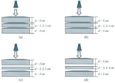
and the central dielectric region are different in each structure. Table 1 lists the bandwidths used for image generation and the corresponding resolutions obtained. Waveforms used for comparison were the Gaussian noiselet and the Mexican Hat wavelet.
(a) (b)
(c) (d)
Figure 9. Defect structures investigated for multiresolution analysis. (a) ST1, (b) ST2, (c) ST3, and (d) ST4.
Table 1. Bandwidths and resolutions investigated.
Frequency range (GHz) Bandwidth (GHz) Depth resolution for εr = 4 (cm)
8–12 4 1.875
8.5–11.5 3 2.5
9–11 2 3.75
9.5–10.5 1 7.5
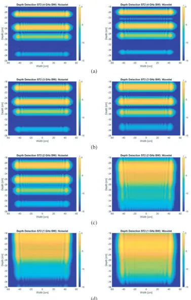
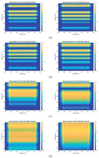
Figures 10–13 show the images obtained for all four structures using both waveforms at different resolutions for structures ST1–ST4, respectively.
From Figs. 10–13, we note that the image resolutions depends on the signal bandwidth for both waveforms. Furthermore, the images get blurred as the resolution degrades by decreasing the bandwidth, as expected [31]. We also note that the images corresponding to each waveform are similar for the same structure at the same resolution.
(a)
(b)
(c)
(d)
(a)
(b)
(c)
(d)
(a)
(b)
(c)
(d)
(a)
(b)
(c)
(d)
show relatively poor results which might be a critical structure for both noiselet and wavelet waveforms to resolve or indicate the structure condition precisely.
Although differences in reconstructed images denote that the noiselet waveform could provide better resolutions or results, we need to quantitatively verify that the noiselet waveform is more advantageous. Moreover, we also need to conform that the frequency bandwidth variation would serve as a powerful potential tool using noiselet waveforms for multiresolution analysis.
6.3. Image Similarity Analysis
To perform multiresolution analysis, we propose an image comparison algorithm to measure the similarity between images at various resolutions. By comparing the correlations between images at different resolutions, it can be assessed whether the degraded image retains or suppresses information relative to the target structure. For this analysis, the raw pixel values were used, not the dB values shown in Figs. 10–13. The notation x(i, j) is used for the reference image and y(i, j) for the image to be compared, where i and j are the location of each measurement point or pixel, and x and y denote the bandwidth in GHz (1–4). Normalization is performed based on following relation to obtain the correlation coefficients Cxy(i, j), given by
Cxy(i, j) =
x(i, j)
y(i, j) ∀x(i, j)< y(i, j)
y(i.j)
x(i, j)∀y(i, j)< x(i, j) 1∀x(i, j) =y(i, j)
(25)
This ensures that the pixel-to-pixel correlation coefficients vary between 0 and 1. The total normalized similarity index between the images, Sxy, is obtained by averaging the pixel-to-pixel correlation
Figure 15. Similarity indices for structure ST2 for different reference images.
coefficients over the entire image, using
Sxy =
∑m j=1
∑n
i=1Cxy(i, j)
m×n (26)
wheremand nare the total numbers of pixels in the two directions of the 2-dimensional image. In our case, m=n= 1024. The similarity factors were obtained by comparing the image data pertaining to 1, 2, 3, and 4 GHz bandwidth signals. Obviously, S11 = S22 = S33 = S44 = 1, and Sxy =Syx. Also, there are a total of six (6) similarity indices with values less than unity.
Figures 14–17 show the similarity indices for structures ST1–ST4, respectively. In these figures, values shown in color depict the largest (red) and the lowest (blue) difference in similarity indices between the values using the noiselet and the wavelet waveforms. We also note that as the bandwidth difference increases, the corresponding similarity index decreases. In general, the similarity indices for the noiselet waveform are higher than that of the wavelet waveform, indicating that the noiselet waveform is better able to associate or relate images at varying resolutions for the same structure.
Figure 17. Similarity indices for structure ST4 for different reference images.
Figures 18 and 19 show the similarity coefficients for the nearest neighbors and the farthest neighbors, respectively. Similarity coefficients for nearest neighbors are S12, S23, and S34, while those for farthest neighbors are S14 (for the 1 and 4 GHz images), S13 (for the 3 GHz image), and S24 (for the 2 GHz image). As can be seen, the nearest neighbor trends show that not much of information is lost when comparing the images of nearest bandwidth pairs. However, the far neighbor trends indicate that the noiselet waveform associates more information between images of differing resolutions when compared to the wavelet waveform.
Figure 18. Similarity coefficient trends for nearest neighbors for various structures.
6.4. Difference Image Analysis
Having established above that the noiselet waveform better preserves structural information across images of varying resolutions, it would be worthwhile to visualize the correlation data to emphasize the area which has more similarity.
(a) (b) (c)
(d) (e) (f)
Figure 20. Difference images for ST1. (a) ∆12, (b) ∆13, (c) ∆14, (d) ∆23, (e) ∆24, and (f) ∆34.
(a) (b) (c)
(d) (e) (f)
(a) (b) (c)
(d) (e) (f)
Figure 22. Difference images for ST3. (a) ∆12, (b) ∆13, (c) ∆14, (d) ∆23, (e) ∆24, and (f) ∆34.
(a) (b) (c)
(d) (e) (f)
Next, the gray scale is applied after normalizing to a 0–255 scale, as follows
∆xy,grayscale = |
∆xy(i, j)|
max|∆xy(i, j)|×255 (28)
Thus, a value of 0 indicates the lowest difference (highest similarity) while a value of 255 indicates highest difference (lowest similarity).
A total of six (6) images are possible for each structure using the four (4) bandwidths, namely, ∆12, ∆13, ∆14, ∆23, ∆24, and ∆34. These six images, converted to grayscale and rendered in color for clarity, were generated for all four structures ST1–ST4. Figs. 20–23 show these images for ST1–ST4, respectively.
The difference mapping of ∆34 provides the best resolution, as expected, due to the combination of larger bandwidths. Interestingly, ∆14 (or even ∆13) results in relatively informative images from which we conclude that the data using a 1-GHz bandwidth noiselet signal can also preserve valuable information about the target.
7. CONCLUSIONS
This paper introduces the concept and applications of noiselet waveforms for multiresolution imaging of various types of defected multilayered structures. The imaging algorithm is developed and tested for imaging of several structural types at different resolutions, high to low. The performance of the noiselet waveform is compared with a traditional wavelet waveform, namely, the Mexican Hat wavelet. It is found that the noiselet better preserves the structural correlations compared to the wavelet, thereby suggesting its advantage over the wavelet for multiresolution analysis. In addition, a modified image difference algorithm developed by us shows promise in exploting the multiresolution images for characterizing the internal features of multilayered structures.
ACKNOWLEDGMENT
This work was supported by the US Office of Naval Research Contract Number N00014-15-1-2021 (POC: William Nickerson).
REFERENCES
1. Coifman, R., F. Geshwind, and Y. Meyer, “Noiselets,” Appl. Comput. Harmon. Anal., Vol. 10, No. 1, 27–44, 2001.
2. Candes, E. and J. Romberg, “Sparsity and incoherence in compressive sampling,” Inverse Prob., Vol. 23, 969–985, 2007.
3. Keep, D. N., “Frequency-modulation radar for use in the mercantile marine,” Proc. IEE — Part B: Radio Electr. Electron., Vol. 103, No. 10, 519–523, 1956.
4. Narayanan, R. M., “Through-wall radar imaging using UWB noise waveforms,” J. Franklin Inst., Vol. 345, No. 6, 659–678, 2008.
5. Ferguson, B., S. Mosel, W. Brodie-Tyrrell, M. Trinkle, and D. Gray, “Characterisation of an L-band digital noise radar,”Proc. 2007 IET International Conf. on Radar Systems, Edinburgh, UK, Oct. 2007, doi: 10.1049/cp:20070634.
6. Axelsson, S. R., “Noise radar using random phase and frequency modulation,” IEEE Trans. on Geoscience and Remote Sensing, Vol. 42, No. 11, 2370–2384, 2004.
7. Foucher, S., G. B. Benie, and J. M. Boucher, “Multiscale MAP filtering of SAR images,” IEEE Trans. Image Process., Vol. 10, No. 1, 49–60, 2001.
8. Graps, A., “An introduction to wavelets,” IEEE Comput. Sci. Eng., Vol. 2, No. 2, 50–61, 1995. 9. Peng, Z. K. and F. L. Chu, “Application of the wavelet transform in machine condition monitoring
12. Rajaraman, P., N. A. Sundaravaradan, R. Meyur, M. J. B. Reddy, and D. K. Mohanta, “Fault classification in transmission lines using wavelet multiresolution analysis,”IEEE Potentials, Vol. 35, No. 1, 38–44, 2016.
13. Rohwer, C., “Multiresolution analysis of sequences,” Nonlinear Smoothing and Multiresolution Analysis, Chapter 7, 71–90, Birkh¨auser Verlag, Basel, Switzerland, 2005.
14. Sadiku, M. N. O., C. Akujuobi, and R. C. Garcia, “An introduction to wavelets in electromagnetics,”IEEE Microwave Mag., Vol. 6, No. 2, 63–72, 2005.
15. Wang, N., Y. Zhang, and S. Wu, “Radar waveform design and target detection using wavelets,”
Proc. 2001 CIE International Conf. on Radar, 506–509, Beijing, China, Oct. 2001.
16. Peele, L. C. and A. N. Pergande, “Wavelet-based radar,” United States Patent No. 5,990,823, 23, Nov. 1999.
17. Wang, L., S. Law, C. Fraker, R. Vela, Y. F. Zheng, R. Ewing, and G. Scalzi, “Development of a new software-defined S-band radar and its use in the test of wavelet-based waveforms,” Proc. 2011 IEEE National Aerospace and Electronics Conf. (NAECON), 162–166, Fairborn, OH, USA, Jul. 2011.
18. Cao, S., Y. F. Zheng, and R. L. Ewing, “Wavelet-based radar waveform adaptable for different operation conditions,”Proc. 10th European Radar Conf., 149–152, Nuremberg, Germany, Oct. 2013. 19. Cao, S., Y. F. Zheng, and R. L. Ewing, “Wavelet-based waveform for effective sidelobe suppression
in radar signal,”IEEE Trans. Aerosp. Electron. Syst., Vol. 50, No. 1, 265–284, 2014.
20. Cao, S., Y. F. Zheng, and R. L. Ewing, “Wavelet-based radar waveform for moving targets detection,” Proc. 2014 IEEE Radar Conf., 1149–1154, Cincinnati, OH, USA, May 2014.
21. Cao, S., Y. F. Zheng, and R. L. Ewing, “Wavelet-based Gaussian waveform for spotlight synthetic aperture radar,”Proc. 2014 IEEE National Aerospace and Electronics Conf. (NAECON), 267–273, Dayton, OH, USA, Jun. 2014.
22. Cao, S., Y. F. Zheng, and R. L. Ewing, “A wavelet-packet-based radar waveform for high resolution in range and velocity detection,”IEEE Trans. Geosci. Remote Sens., Vol. 53, No. 1, 229–243, 2015. 23. Sullivan, E. J., R. P. Goddard, H. A. Greenbaum, and K. P. Bongiovanni, “Generating simulated
reverberation using noiselets,” J. Acoust. Soc. Am., Vol. 119, No. 5, Pt. 2, 3273, 2006.
24. Matsumoto, M. and N. Takuji, “Mersenne twister: A 623-dimensionally equidistributed uniform pseudo-random number generator,”ACM Trans. Model. Comput. Simul. (TOMACS), Vol. 8, No. 1, 3–30, 1998.
25. Balanis, C. A.,Advanced Engineering Electromagnetics, John Wiley & Sons, New York, NY, USA, 1999.
26. Richards, M. A., Fundamentals of Radar Signal Processing, McGraw-Hill, New York, NY, USA, 2005.
27. Martinez-Lorenzo, J. A., F. Quivira, and C. M. Rappaport, “SAR imaging of suicide bombers wearing concealed explosive threats,” Progress In Electromagnetics Research, Vol. 125, 255–272, 2012.
28. Dehmollaian, M., and K. Sarabandi, “Refocusing through building walls using synthetic aperture radar,”IEEE Trans. Geosci. Remote Sens., Vol. 46, No. 6, 1589–1599, 2008.
29. Stolt, R. H., “Migration by Fourier transform,” Geophys., Vol. 43, No. 1, 23–48, 1978.
30. Lopez-Sanchez, J. M. and J. Fortuny-Guasch, “3-D radar imaging using range migration techniques,” IEEE Trans. Antennas Propag., Vol. 48, No. 5, 728–737, 2000.