IMPACTS OVER KENYA
Philip Obaigwa Sagero (M.Sc.)
Thesis submitted in Fulfillment of the Requirements for the Award of the Degree of Doctor of Philosophy in Climatology in the School of Pure and Applied Science,
Kenyatta University.
DECLARATION
This thesis is my original work and has not been presented for a degree in any other university or any other award.
Signature……… Date....………. Philip Obaigwa Sagero
I84/30690/2015
Department of Geography,
School of Pure and Applied Science Kenyatta University
Supervisors
We confirm that the candidate carried out the work reported in this thesis under our supervision
Signature………. Date……… Prof. Chris A. Shisanya (Ph.D.)
Geography Department Kenyatta University
Signature………. Date………
Dr. George L. Makokha (Ph.D.) Geography Department
DEDICATION
ACKNOWLEDGMENTS
I am highly grateful to God who bestowed me with good health and strength to go through my entire education and completion of this Doctorate thesis.
It is an honor to express my appreciation to my supervisors Prof. Chris A. Shisanya and Dr. George L. Makokha of Geography Department for their guidance, constructive criticism, support and their time to read and scrutinize my work that leads to the timely completion of my studies. I also acknowledge the management of department of Geography, Kenyatta University for facilitating the training.
I also extend my appreciation to the Director Kenya Meteorological Department (KMD), under the Ministry of Environment and Forestry for granting me study leave that gave me ample time to pursue my studies and colleagues at KMD for also understanding during the time I was away.
TABLE OF CONTENTS
DECLARATION ... ii
DEDICATION ... iii
ACKNOWLEDGMENTS ... iv
LIST OF TABLES ... viii
LIST OF FIGURES ... x
LIST OF ACRONYMS AND ABBREVIATIONS ... xvi
ABSTRACT ... xviii
CHAPTER ONE ... 1
INTRODUCTION ... 1
1.1 Background to the study problem ... 1
1.2 Statement of the Problem ... 4
1. 3 Research Questions ... 6
1.4 Null Hypothesis ... 6
1.5 Objectives of the Study ... 7
1.5.1 General Objective ... 7
1.5.2 Specific Objectives ... 7
1.6 Significance and Justification of the Study... 7
1.7 Scope and Limitation of the study ... 8
1.8 Overview of the Thesis ... 9
CHAPTER TWO ... 11
LITERATURE REVIEW ... 11
2.1 Introduction... 11
2.2 Rainfall and Temperature Trend over Kenya ... 11
2.3 Systems and Processes that Influence Rainfall Distribution over Kenya... 13
2.3.1 Inter-Tropical Convergence Zone (ITCZ) ... 13
2.3.2 Tropical Cyclones ... 14
2.3.3 Subtropical Anticyclone ... 14
2.3.4 Monsoon ... 15
2.3.5 Jet Streams ... 16
2.3.6 Quasi-Biennial Oscillations ... 16
2.3.8 El Niño Southern Oscillation (ENSO) ... 17
2.3.9 Indian Ocean Dipole ... 18
2.4 Climate Models and Climate Systems ... 19
2.5 Changes in Rainfall and Temperature Extremes ... 21
2.6 Impacts of Climate Change and variability ... 23
2.6.1 Agriculture ... 24
2.6.2 Water ... 26
2.6.3 Health ... 27
2.6.4 Energy ... 28
2.6.5 Urbanization... 29
2.7 Policies and Institutional Frameworks for Coping with Climate Change ... 31
2.8 Conceptual Model ... 34
CHAPTER THREE ... 35
MATERIAL AND METHODS ... 35
3.1 Study Area ... 35
3.1.1 Climatology of the Study Area ... 36
3.2 Data ... 38
3.2.1 Observed Station Data... 39
3.2.2 Gridded Datasets ... 39
3.2.3 Sea Surface Temperature ... 43
3.2.4 Coordinated Downscaled Experiment Datasets ... 43
3.3. Methodology ... 47
3.3.1 Missing Data and Quality Control ... 47
3.3.2 Determination of Spatial-Temporal Variability, Pattern, and Trend of Rainfall and Temperature ... 48
3.3.3 Evaluate the Performance of the CORDEX RCMs in Simulating the Observed Rainfall and Temperature Variability. ... 52
3.3.4 Evaluation of the CORDEX RCMs in Capturing the Influence of Large-Scale Circulation (Teleconnection) Signals in Kenyan Rainfall ... 53
3.3.6 Analysis of Future Changes in Rainfall and Temperature Extremes ... 54
3.3.7 Analysis of Probability Density Function (PDFs) ... 55
3.3.7 Analysis of the Likely Impacts ... 57
CHAPTER FOUR ... 58
RESULTS AND DISCUSSION ... 58
4.2 Homogeneity Test ... 58
4.3 Rainfall and Temperature Pattern, Variability and Trend ... 59
4.3.1 Spatial-Temporal Rainfall Pattern and Variability ... 59
4.3.2 Spatial-Temporal Temperature Pattern ... 70
4.3.3. Rainfall Trend Analysis ... 79
4.3.4 Temperature Trend Analysis ... 87
4.4 Assessing the Ability of the RCMs in Simulating the Rainfall and Temperature 94 4.5 Assessment of the RCMs’ Skills in Simulating Large-Scale Signals ... 104
4.6 Analysis of Future Projections of Temperature and Rainfall over Kenya ... 117
4.6.1 Changes in Future Rainfall under RCP 4.5 and RCP8.5 Scenarios over Kenya. .... 119
4.6.2 Future Temperature Change over Kenya. ... 138
4.6.3 Simulated Future Change in Climate Extreme Events over Kenya ... 144
4.7 The likely Sectorial Impacts of the Projected Rainfall and Temperature Change ... 152
4.7.1 Agriculture Sector ... 156
4.7.2 Water resource... 159
4.7.3 Health ... 159
4.7.3 Energy ... 160
4.7.4 Urbanization... 160
CHAPTER FIVE ... 162
SUMMARY OF FINDINGS, CONCLUSIONS AND RECOMMENDATIONS ... 162
5.1 Introduction... 162
5.2 Summary of Findings ... 163
5.3 Conclusions ... 165
5.4 Recommendations ... 166
5.5 Suggested Further Research ... 168
6 REFERENCES ... 170
LIST OF TABLES
Table 3. 1: Summary of the data used in the study ... 38 Table 3. 2: Name, position, Elevation and Data length of the rainfall observation
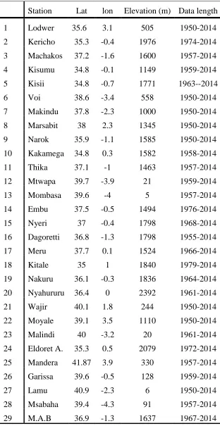
stations used in the study ... 42 Table 3. 3: List of CORDEX RCMs and their details (Source; Nikulin et al.,
2012) ... 45 Table 3. 4: Definition of extreme temperature and rainfall indices used in this
study ... 56 Table 3. 5: Guide for Impact analysis ... 57
Table 4. 1: Summary of correlation c o e f f i c i e n t and R oot M ean S quare Error ( RMSE) between GPCC, CRU and observed station data over Kenya ... 61 Table 4. 2: Annual and seasonal (MAM and OND) means (mm) for 33 stations
and their percentage (%) contribution to the Annual rainfall for
1960-2014. ... 66 Table 4. 3: The Mean, Standard deviation and Coefficient of Variability (CV) for
March-April-May (MAM), October-November-December (OND) and Annual rainfall ... 69 Table 4. 4: Statistics of Seasonal mean (µ) and standard deviation (σ) of Tmax
for various stations for 1950 -2014 ... 77 Table 4. 5: Statistics of the Seasonal mean (µ) and standard deviation (σ) of Tmin
for various stations for 1960-2014 ... 78 Table 4. 6: Mann-Kendall (MK) statistics, Sen’s slope and P-value for MAM,
OND and Annual for different station (highlighted in red show statistically significant at 5% level) ... 86 Table 4. 7: Mann-Kendall trend test results for Tmin (Z and p-value) and the
slope S. ... 90 Table 4. 8:Mann-Kendall trend test results for Tmax (Z and p-value) and the slope
Table 4. 9: Summary of RMSE between GPCC, CRU and CORDEX RCMs data over Kenya ... 99 Table 4. 10: Summary of co rr el at i on between GPCC, CRU and CORDEX
RCMs data over Kenya ... 99 Table 4. 11: The years of IOD, ENSO and the co-occurrence of both ... 107 Table 4. 12: Rainfall stations used for each Homogeneous zone in the Study and
their Coordinates for (a) MAM and (b) OND Seasons ... 119 Table 4. 13: Results of Mann-Kendall test statistic for rainfall over Kenya for the
period of 2021–2100 for the five CORDEX models (a) MAM and (b) OND (c) Annual (** for trend at α = 0.01 level of significance, * if trend at α = 0.05 level of significance, + for trend at α = 0.1 level of significance, If the cell is blank, the trend is insignificance at level less than 0.1) ... 132 Table 4. 14: Results of the Mann-Kendall test statistic and sen’s slope for MAM
seasonal rainfall over Kenya homogeneous rainfall zones for the period of 2021–2100 (** for trend at α = 0.01 level of significance, * if trend at α = 0.05 level of significance, + for trend at α = 0.1 level of significance, If the cell is blank, the trend is insignificance at level less than 0.1). ... 134 Table 4. 15: Results of the Mann-Kendall test statistic and sen’s slope for OND
seasonal rainfall over Kenya homogeneous rainfall zones for the period of 2021–2100 (** for trend at α = 0.01 level of significance, * if trend at α = 0.05 level of significance, + for trend at α = 0.1 level of significance, If the cell is blank, the trend is insignificance at level less than 0.1). ... 135 Table 4. 16: Summary of the MK test statistic and sen’s slope for seasonal
maximum and minimum temperature over Kenya for the period of 2006–2100 at α = 0.01 level of significance under the RCP4.5 and RCP8.5 scenarios. ... 144 Table 4. 17: Results of Mann-Kendall and Sen’s slope for temperature and
rainfall indices for a period of 1971 to2100, with base period of
1971-2005 for RPC 4.5 ... 150 Table 4. 18:Results of Mann-Kendall and Sen’s slope for temperature and rainfall
LIST OF FIGURES
Figure 2. 1: SST anomalies (red shading denotes warming; blue-cooling) during (a) El Niño and (b) La Niña events (source: NOAA/ National Weather Service) ... 18 Figure 2. 2: SST anomalies (red shading is for warm anomalies and blue for cold).
White patches indicate increased convective activities and arrows indicate anomalous wind directions during (a) positive and (b) negative Indian Ocean Dipole events. (Source: Japan Agency for Marine-Earth Science and Technology) ... 19 Figure 2. 3: A diagram of an Urban Heat Island – Temperatures in the city Centre
are a few degrees warmer compared to the city’s periphery (Source: EPA, 2008 Quoted in http://www.urbanheatislands.com/ Accessed 18 April 2019) ... 30 Figure 2. 4: Conceptual Model (Source; Author, 2018) ... 34
Figure 3. 1: Map of Kenya showing Kenyan counties, water bodies and rainfall stations used in the study. ... 37
Figure 4. 1: Cumulative plot of annual rainfall (mm) showing homogeneity of
the rainfall data from three stations in Kenya. ... 58 Figure 4. 2: Climatology of annual rainfall over Kenya for station observed,
CRU and GPCC (1960-2014) ... 60 Figure 4. 3: Climatology of MAM rainfall season over Kenya for station
observed, CRU and GPCC (1960-2014) ... 60 Figure 4. 4: Climatology of OND rainfall season over Kenya for station
observed, CRU and GPCC (1960-2014) ... 61 Figure 4. 5: Annual rainfall cycle over Kenya form the Observed station data,
GPCC and CRU datasets ... 62 Figure 4. 6: Time series of seasonal rainfall (a) MAM season (b) OND season
for the observed, CRU and GPCC datasets over Kenya. ... 63 Figure 4. 7: The average annual cycles of rainfall for selected station (Moyale,
Figure 4. 8: Annual temperature cycle over Kenya for (a) Minimum (b) Maximum, where the red line show station observed data and blue
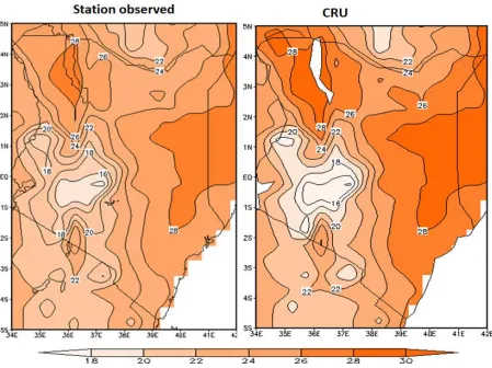
for CRU data ... 71 Figure 4. 9: Climatology of mean temperature over Kenya based on station
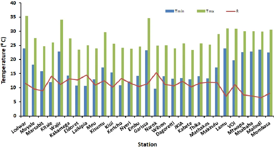
observed and CRU datasets for (1980-2014). ... 72 Figure 4. 10: Mean maximum temperature (Tmx), minimum temperature
(Tmin) and temperature range (R) for the various stations over
Kenya ... 73 Figure 4. 11: Temperature range Monthly climatology (°C) over Kenya for
January – December) based on the CRU datasets for 1970 – 2015.
... 75 Figure 4. 12: Decadal change in March-May rainfall anomaly from 1901 to
2010 relative to the base period of 1981 – 2010 over Kenya based
on CRU datasets ... 80 Figure 4. 13: Decadal change in March-May rainfall anomaly from 1901 to
2010 relative to the base period of 1981 – 2010 over Kenya based
on GPCC datasets ... 81 Figure 4. 14: Decadal change in October-December rainfall anomaly from 1901
to 2010 relative to the base period of 1981 – 2010 over Kenya
based on CRU datasets ... 82 Figure 4. 15: Decadal change in October-December rainfall anomaly from 1901
to 2010 relative to the base period of 1981 – 2010 over Kenya
based on GPCC datasets ... 83 Figure 4. 16: Spatial distribution of Mann-Kendall (MK) at 5% level of
significance statistics for (a) MAM, (b) OND and (c) Annual ... 85 Figure 4. 17: Abrupt change in annual rainfall over Kenya where the red is for
forward sequential, blue is for backward sequential statistic and
the dashed lines represent the confidence limits at 5%. ... 87 Figure 4. 18: Spatial Distribution of monthly Man-Kendall (MKZ)statistics for
Tmax for 1960 – 2014 ... 93 Figure 4. 19: Spatial Distribution of Monthly Man-Kendall (MKZ) statistics for
Figure 4. 20: Climatology (1971-2005)) of rainfall during MAM season over Kenya as simulated by 8 CORDEX RCMs, GPCC and CRU
datasets. ... 96 Figure 4. 21: Climatology of rainfall during OND season as simulated by 8
CORDEX RCMs, GPCC, and CRU over Kenya. ... 97 Figure 4. 22: Mean annual cycle of rainfall over Kenya (mm/day) from the
CRU, GPCC, and the 8 CORDEX RCMs ... 98 Figure 4. 23:Time series of the inter-annual variability of annual rainfall in
CORDEX models and the observed (CRU and GPCC) in terms of
their anomalies (mm) ... 100 Figure 4. 24: December – February average (1971-2005) seasonal temperature
for CORDEX models and the observed (CRU) ... 101 Figure 4. 25: March-May average (1971-2005) temperature for CORDEX
models and the observed (CRU) ... 102 Figure 4. 26: June-August average (1971-2005) temperature for CORDEX
models and the observed (CRU) ... 103 Figure 4. 27: Mean annual cycles of Temperature simulated by the observed
(CRU) and CORDEX models during the period 1971-2000. ... 104 Figure 4. 28: Graphical depictions of the four Niño regions (source: CPC:
http://www.cpc.noaa.gov/products/analysis_monitoring/ensostuff
/ninoregions.shtml) ... 106 Figure 4. 29:Index of IOD and Nino 3.4 during January 1960 to December 2016
period. Positive (Negative) Anomaly Shows El Niño (La Niña)
event and Positive (Negative) IOD. ... 106 Figure 4. 30: Variation of monthly mean NINO 3.4 and DMI for co-occurring
event years (1982, and 1997), where (-1) indicate year before, (0)
year when it occurred and (+1) year after it has occurred. ... 107 Figure 4. 31: Composite of SST anomaly (oC) during OND and MAM, on (a)
Positive IOD, (b) Negative IOD, (c) El Niño, (d) La Niña (e) Positive IOD and El Niño, (f) Negative IOD and La Niña, and (g) No IOD and No ENSO. Positive (negative) value shows the
increasing (decreasing) of SSTs. ... 109 Figure 4. 32: Spatial correlation of Kenyan rainfall to the Sea surface
Figure 4. 33: Composite rainfall anomalies during MAM season for CRU and
GPCC data for the classification years listed in (Table 4.11). ... 111 Figure 4. 34: Composite rainfall anomalies during OND season for CRU and
GPCC data for the classification years listed in (Table 4.11). ... 112 Figure 4. 35: Correlation results of the model mean rainfall with that of IOD
and NINO 3.4 ... 113 Figure 4. 36: Composite of simulation of precipitation anomalies during OND
season of pure El Niño years ... 114 Figure 4. 37: Composite of simulation of precipitation anomalies during OND
season of co-occurrence of El Niño and positive IOD years ... 115 Figure 4. 38: Composite of simulation of precipitation anomalies during OND
season of La Niña years ... 116 Figure 4. 39: Composite of simulation of precipitation anomalies during OND
season of co-occurrence of La Niño and negative IOD years ... 117 Figure 4. 40: Homogeneous rainfall zones over Kenya for (a) MAM and (b)
OND seasons. Source: Rainfall Atlas (Authors: Muhindi, Ndichu,
and Oloo, Kenya Meteorological Dept, 2001) ... 118 Figure 4. 41: March-May seasonal rainfall change (mm) over Kenya as
simulated by RACMO model under the RCP4.5 scenario, relative
to the baseline period 1961–2000. ... 120 Figure 4. 42: March-May seasonal rainfall change (mm) over Kenya as
simulated by RACMO model under the RCP8.5 scenario, relative
to the baseline period 1961–2000. ... 121 Figure 4. 43:March-May seasonal rainfall change (mm) over Kenya as
simulated by CCLM model under the RCP4.5 scenario, relative to
the baseline period 1961–2000. ... 121 Figure 4. 44: March-May seasonal rainfall change (mm) over Kenya as
simulated by CCLM model under the RCP8.5 scenario, relative to
the baseline period 1961–2000. ... 122 Figure 4. 45: March-May seasonal rainfall change (mm) over Kenya as
simulated by HIRHAM model under the RCP4.5 scenario, relative
Figure 4. 46: March-May seasonal rainfall change (mm) over Kenya as simulated by HIRHAM model under the RCP8.5 scenario, relative
to the baseline period 1961–2000. ... 123 Figure 4. 47: March-May seasonal rainfall change (mm) over Kenya as
simulated by RCA model under the RCP4.5 scenario, relative to
the baseline period 1961–2000. ... 123 Figure 4. 48: March-May seasonal rainfall change (mm) over Kenya as
simulated by RCA model under the RCP8.5 scenario, relative to
the baseline period 1961–2000. ... 124 Figure 4. 49: March-May seasonal rainfall change (mm) over Kenya as
simulated by REMO model under the RCP4.5 scenario, relative to
the baseline period 1961–2000. ... 124 Figure 4. 50: March-May seasonal rainfall change (mm) over Kenya as
simulated by REMO model under the RCP8.5 scenario, relative to
the baseline period 1961–2000. ... 125 Figure 4. 51: October-December seasonal rainfall change (mm) over Kenya as
simulated by RACMO model under the RCP4.5 scenario, relative
to the baseline period 1961–2000. ... 126 Figure 4. 52: October-December seasonal rainfall change (mm) over Kenya as
simulated by RACMO model under the RCP8.5 scenario, relative
to the baseline period 1961–2000. ... 126 Figure 4. 53: October-December seasonal rainfall change (mm) over Kenya as
simulated by CCLM model under the RCP4.5 scenario, relative to
the baseline period 1961–2000. ... 127 Figure 4. 54: October-December seasonal rainfall change (mm) over Kenya as
simulated by CCLM model under the RCP8.5 scenario, relative to
the baseline period 1961–2000. ... 127 Figure 4. 55: October-December seasonal rainfall change (mm) over Kenya as
simulated by HIRHAM model under the RCP4.5 scenario, relative
to the baseline period 1961–2000. ... 128 Figure 4. 56: October-December seasonal rainfall change (mm) over Kenya as
simulated by HIRHAM model under the RCP8.5 scenario, relative
Figure 4. 57: October-December seasonal rainfall change (mm) over Kenya as simulated by RCA model under the RCP4.5 scenario, relative to
the baseline period 1961–2000. ... 129 Figure 4. 58: October-December seasonal rainfall change (mm) over Kenya as
simulated by RCA model under the RCP8.5 scenario, relative to
the baseline period 1961–2000. ... 129 Figure 4. 59: October-December seasonal rainfall change over Kenya as
simulated by REMO model under the RCP4.5 scenario, relative to
the baseline period of 1961–2000. ... 130 Figure 4. 60: October-December seasonal rainfall (mm) change over Kenya as
simulated by REMO model under scenario RCP8.5, relative to the
baseline period 1961–2000. ... 130 Figure 4. 61: Probability Density Function for MAM seasonal rainfall under
RCP4.5 and RCP8.5 scenarios [RCP4.5 (blue) and RCP8.5 (red)] for 2061–2100 and (black) baseline period for 1961–2000. 1–12
represent homogeneous regions 1–12, respectively ... 136 Figure 4. 62: Probability Density Function for OND seasonal rainfall under
RCP4.5 and RCP8.5 scenarios [RCP4.5 (blue) and RCP8.5 (red)] for 2061–2100 and (black) baseline period for 1961–2000. 1–12
represent homogeneous regions 1–12, respectively ... 137 Figure 4. 63: Maximum temperature change (°C) projected by ensembled
model under RCP4.5. ... 139 Figure 4. 64: Maximum temperature change (°C) projected by ensembled
model under RCP8.5. ... 140 Figure 4. 65: Minimum temperature change (°C) as projected by ensembled
model under RCP4.5. ... 141 Figure 4. 66: Minimum temperature change (°C) as projected by ensembled
Model under RCP8.5. ... 142 Figure 4. 67: Probability Density Functions for the mean annual temperature
under different RCP4.5 and 8.5 scenarios over Kenya. ... 143 Figure 4. 68: Annual time series of temperature extremes for Kenya as
predicted by the three CCLM, HIRHAM, and RACMO RCMs. ... 146 Figure 4. 69: Annual time series of rainfall extremes for Kenya as predicted by
LIST OF ACRONYMS AND ABBREVIATIONS AR5 Fifth Assessment Reports
COP Conference of Parties
CORDEX Coordinated Regional Climate Downscaling Experiment CRU Climate Research Unit
EA East Africa
ENSO El Niño–Southern Oscillation EALLJ East Africa Low Level Jet
ETCCDI Expert Team on Climate Change Detection and Indices GCMs Global Climate Models
GHG Green House Gases GHA Great Horn of Africa
GPCC Global Precipitation Climatology Centre GDP Gross Domestic Product
IOD Indian Ocean Dipole
IPCC Intergovernmental Panel on Climate Change ITCZ Inter-Tropical Convergence Zone
JJA June July August
KM Kilometers
MAM March April May
NE Northeast
OND October November December
R99p Annual total PRCP when RR > 99thpercentile RACMO2 Regional Atmospheric Climate Model RCMs Regional Climate Models
RCPs Representative Concentration Pathways RMSE Root Mean Square Error
RVF Rift Valley Fever SE Southeast
SEI Stockholm Environment Institute SST Sea Surface Temperatures
TMAXmean Annual mean maximum temperature TMINmean Annual mean minimum temperature
TNx Monthly maximum value of daily minimum temp TRMM Tropical Rainfall Measuring Mission
TXx Monthly maximum value of daily maximum temp UNFCC United Nation Framework on Climate Change WCRP World Climate Research Program
WHO World Health Organization
WMO World Meteorological Organization
NCCRS National Climate Change Response Strategy NCCAP National Climate Change Action Plan
ABSTRACT
CHAPTER ONE INTRODUCTION 1.1 Background to the study problem
Climate change and variability is the most pressing environmental and development challenge facing most countries today (Conway, 2009). Countries will be affected differently by the projected change in climate and therefore each country requires different adaptive and mitigation strategies (Vincent, 2007). At the end of 21st century, the global temperature is projected to increase by 1.4 to 5.8 oC (IPCC, 2014). Global warming will likely change the weather patterns around the globe (IPCC, 2007; Stern, 2006). Africa is the most affected continent by climate change, and it is a threat to its economic growth, long-term prosperity, as well as the survival of already vulnerable populations. This is because of low adaptative capacity due to lack of enough resources. Understanding the projected future climate scenarios at seasonal, annual, decadal and multi-decadal variations in climate change and variability has become the major challenge facing scientists in most of African countries in recent years (Hulme et al., 2001).
and 4 oC by the end of twenty-first century (Niang et al., 2014), with little mitigation measures and adaptation strategies to the changes, the impacts on livelihood of the local communities caused by climate change are likely to increase.
According to Nzau (2013), Kenya is also experiencing the impacts of climate change. It is costing Kenya 2.4% of its Gross Domestic Product (GDP). He further states that; climate variability and change is impacting many sectors of the economy and there is a need for diversification at both national and local level to reduce on reliance on rainfed agriculture as the main source of livelihood for the local communities across Kenya. The agricultural sector is one of the major economic activity in Kenya, which accounts for about 30% of the GDP and 60% foreign exchange earner. It also forms the main source of employment (ICPAC, 2006). Some of the other sectors of the economy that are climate depended include; livestock keeping, hydro-energy generation, transport, and tourism. 60% of socio-economic activities are dependent on climate (WRI et al., 2007). Climate extreme such as floods and droughts have a high influence on the social-economic activities of the country and thus also affect performance of the country’s economy (GOK, 2013). Thus, understanding climate variability and change and its future scenario at a local scale is very important for economic growth and formulation of adaptation strategies that will increase the resilient of the local community.
vulnerability level of the community at local scale.
In order to increase resilient and reduce the vulnerability of the society, it is important to understand past and future climate variability and change and its extremes. Climate models are used for simulation of the past and future climate to explore the possible change in future climate. The most common approach of simulating the future climate scenario is by use of Global Climate Models (GCMs). The GCMs have a coarse resolution of more than 100 km, this constrains them from capturing the effects of local climate forcing such as Land–sea contrast and terrain effects that modulate climate at finer scales. It also limits them to reproduce the extreme events that are mostly localized and which are important in impact assessment at the local scale (Giorgi, 1990).
able to simulate large-scale features, they are a suitable tool for assessing the past and future climate change over Kenya. Studies by Nikulin et al. (2012), Endris et al. (2013) and Omondi et al. (2014) have proven that RCMs are a suitable tool for simulation of future climate over East Africa for impact assessment. Most of these studies are mainly covering the East African region or the Great Horn of Africa (GHA). Given the heterogeneity and complexity of East Africa, small-scale analysis of climate change simulated by RCMs is necessary. This study attempted to bridge the gap by use of multiple RCMs simulation driven by different GCMs to assess the ability to reproduce rainfall and temperature pattern over Kenya. This study, therefore, intends to review the past and present temperature and rainfall pattern and changes over Kenya and investigate future projection of both mean and extreme temperature and rainfall under increase Representative Concentration Pathways (RCPs) 4.5 and 8.5.
1.2 Statement of the Problem
Effects of climate variability and change are being felt in East Africa and Kenya is one of the most vulnerable countries to climate variability and climate change (IPCC, 2014). Climate extremes such as drought and floods have become more frequent in Kenya and are projected to increase in intensity and frequency (Niang et al., 2014). The two extreme events are associated with social-economic loses. For example, the two recent droughts 2008-2009 and 2010-2011 in Kenya affected millions of people. According to IPCC (2007), the African continent has warmed by 0.5 oC and the annual temperatures are
majorly depend on rain-fed agriculture unless adequate adaptation strategies are developed. Climate change will reduce productivity of rain-fed agriculture, increase widespread shortage of clean drinking water and significantly increase in crop, livestock and human diseases (Jones and Thornton, 2003). Therefore, it is important to understand climate variability and change in Kenya to help minimize the potential impact of climate related loss by developing better adaptation strategies.
Although IPCC reports provide a good indication of the possible magnitude of climate change by use of GCMs, there are several shortcomings in the use of this information for local impact assessment and development of adaptation measures. GCMs can satisfactorily simulate the synoptic systems, but they are not capable of capturing detailed processes associated with local climate variability and changes that are required for assessing the impacts of climate change at local scale (Wang et al., 2004). Hence, their outputs are not useful in the development of adaptation strategies to reduce the impact of future climate change at the household level.
This study will attempt to overcome these shortcomings by considering multiple RCMs simulations which have been nested on different GCMs that are used in the preparation of IPCC reports and assess their ability to reproduce the local scale climate variability and change over Kenya. Then further investigate the future change in climate in both spatial and temporal scale under RCPs 4.5 and 8.5. This will result in a comprehensive future
climate change scenario for Kenya at a high resolution that is required for building a
resilient society and economy in support of national disaster risk reduction, climate change
of climate change at local scale.
1. 3 Research Questions
The study was guided by the following questions:
i. What are the spatiotemporal patterns and trends of rainfall and temperature in Kenya?
ii. Do regional climate models reproduce the rainfall and temperature pattern over Kenya?
iii. Are the regional climate models able to capture the teleconnection associated with Kenyan Rainfall?
iv. What are the possible future changes in rainfall and temperature extremes under Representative Concentration Pathways (RCPs) 4.5 and 8.5 over Kenya?
v. What are the likely impacts of projected change in rainfall and temperature in Kenya?
1.4 Null Hypothesis
i. There is no significant increase in temperature over Kenya
ii. There is no significan increase in rainfall over Kenya iii. The RCMs do not significantly reproduce the observed rainfall and temperature
1.5 Objectives of the Study
1.5.1 General Objective
This study assessed the ability of regional climate models in simulating observed rainfall and temperature patterns and projecting the future climate scenario for impact assessment over Kenya.
1.5.2 Specific Objectives
i. To determine rainfall and temperature spatiotemporal patterns, variability and trends for a period 1901 to 2014 over Kenya
ii. To evaluate the performance of the regional climate models in simulating the rainfall and temperature patterns in Kenya
iii. To evaluate the ability of the regional climate models in assimilating the large-scale climate circulation (teleconnection) that influence rainfall over Kenya iv. To determine the future changes in rainfall and temperature extremes under
Representative Concentration Pathways (RCPs) 4.5 and 8.5.
v. To analyze the likely impacts of the projected rainfall and temperature change 1.6 Significance and Justification of the Study
global models. The analysis of climate change at small scale, especially at country level and understand the climate variability and change is limited. There is great interest in assessing the impacts of projected climate change, and more specifically, the impacts of the change in variability and extreme events that could accompany the global warming (Tebaldi et al., 2006). To do these impacts studies at the local scale, appropriate high-resolution models that can simulate the local and large-scale features that affect the climate of a region must be used.
Given that households are particularly vulnerable to extreme climatic events such as flooding and drought, accurate estimate of local changes in precipitation and temperature are valuable for informing local policy decisions and estimating potential impacts on all areas of the economy such as health, infrastructure, ecosystems and agriculture (Sun et al., 2006). Therefore, this study contributes to the understanding of the past and future climate variability and the information will help in understanding some of the impacts on society and the ecosystem. The policymakers, investors, planners and even communities need this information on the future climate change so that they can prepare for the expected trend and change. The availability of this climate information is also critical in mainstreaming climate change into national and county policy-making processes. It will also greatly benefit the modeling community on the strength and weakness of their models, which will help improve them in the future.
1.7 Scope and Limitation of the study
another element such as humidity, wind, sunshine, and evaporation which are also critical in climate analysis. Thus, climate variability in this study is limited to rainfall and temperature because they are the most important variable used in climate change studies.
The study also used only the manned Kenya meteorological synoptic station, that spread throughout the country. Several other voluntary stations were left out due to the quality and gaps in data from some of the stations. Due to the expansive nature of the country and it’s known spatial variability in rainfall and temperature, 12 climatological zones were used to represent each region in the country. Each station had also different length of period, this was because the stations were opened at different time. The study also used station data which is point data to compare with that of gridded data. No bias correction was done to the RCMs data used in the assessment of the future climate projection for Kenya for lack of computing facility, nevertheless, comparison was done with the observed gridded data. The study considered only two RCPs 4.5 and 8.5 out of the four available RCPs. This is because of the availability of RCMs data. Five sectors were used in the analysis of the likely impacts of the projected climate change. The sectors were identified as the most impacted through literature and also no models were used.
1.8 Overview of the Thesis
CHAPTER TWO LITERATURE REVIEW 2.1 Introduction
Several studies have been carried out in an effort to understand climate change and climate variability over Kenya. In the recent past studies aimed at assessing climate models and their effectiveness in simulating the East African weather have been on increase. This chapter reviews some of the studies that have been carried out over East Africa and other regions which are relevant to this study.
2.2 Rainfall and Temperature Trend over Kenya
Understanding rainfall and temperature trends have become a very important aspect of
climate research study; it helps to clarify climate change discourse and its effect on society
and ecosystems. East Africa is one of the regions that are highly vulnerable to the effects
of climate change owing to a number of reasons ranging from natural, technology to
economic (IPCC, 2007). Thus, reliable and timely climate information on the future climate
changes is needed to avert the negative impacts associated with the changes. Several
studies have been carried at different scale on rainfall and temperature trends across Eastern
Africa region (Nicholson, 2000; Hulme et al., 2001; Schreck and Semazzi, 2004; Mwangi
and Desanker, 2007; Makokha and Shisanya, 2010; Moyo et al., 2012; Wagesho et al., 2013; Opiyo et al., 2014). They have revealed that there have been changes that have
occurred in rainfall and temperature in the East Africa region. It is also projections that by
Studies show that the region is currently experiencing an increase in October -December
(OND) rainfall and reduction in March-May (MAM) rainfall (Liebmann et al., 2014;
Ongoma and Chen, 2017). While Shongwe et al. (2011) and Otieno and Anyah (2013)
report there is a likelihood of an increase in MAM rainfall at the end of 21st century. So,
there is uncertainty owing to the current observation over East Africa. On the other hand,
studies on temperature observation show significantly increasing trends, in the frequency
of warm days and larger increasing trends in the frequency of warm nights (Omondi et al.,
2012). However, WWF (2006) argues that the average number of warm days per annuum
has increased by 57% between 1960 and 2003. The rate of increase is seen mostly during
the MAM season, when the average number of hot days increased significantly by 5.8 days
per month thus an additional 18.8% of MAM hot days over this period. Other studies
indicate that the mean annual temperatures have increased by 1.0 °C since 1960, or an
average rate of 0.21 °C per decade in Kenya (McSweeney et al., 2009).
Rainfall pattern changes have also been noticed since the 1960s. Increased rainfall has been
observed during the October to December rainfall season (Ongoma et al., 2017) while
decreasing during the March to May season. The March to May rainfall which is the long
rain season, has become increasingly unreliable in some part of Kenya (Awuor et al.,
2.3 Systems and Processes that Influence Rainfall Distribution over Kenya
In the study of climate change and climate variability, it is important to understand the systems that influence weather and climate patterns over the study area. Spatiotemporal variability of rainfall and temperature in Kenya is influenced by several systems. These systems are global, regional and local and interact in a complex way at various spatial and temporal scale to bring about the variability in rainfall and temperature. Some of the synoptic and mesoscale scale systems that affect the weather and climate over Kenya are briefly discussed in the next subsections.
2.3.1 Inter-Tropical Convergence Zone (ITCZ)
fluctuation of rainfall amount and distribution are attributed to the anomalies in the large-scale factors that influence the characteristic of the ITCZ over Est Africa region.
2.3.2 Tropical Cyclones
A tropical cyclone is an intense spiral storm that occurs in warm tropical Ocean and is characterized by low pressure, heavy rainfall and strong winds. The cyclones that affect the weather in Kenya are those that form over the South Western Indian Ocean. They normally form from November to May, their influence on Kenyan weather is not directly linked. Their effect depends on their track and time of occurrence, their formation during late March and earlier April often leads to delay and below normal long rainfall over Kenya during MAM season (Okoola, 1999).
2.3.3 Subtropical Anticyclone
over land as compared to SE which is long and over the ocean resulting in lesser rainfall during the OND season. On the other hand, During March-May (MAM) season, Mascarene is more intense than Arabian high driving strong SE which their trajectory through the ocean toward East Africa region. The convergences of SE and NE caused by the ITCZ result in more rainfall during the MAM season. The influence of St. Helena high is determined by the position of the meridional arm of the ITCZ which determine the convergence of westerlies and easterlies.
2.3.4 Monsoon
2.3.5 Jet Streams
Jet stream is a narrow fast flowing wind. They form at the boundary of two of adjacent air masses with the difference in temperature. Over Kenya, there are two jet streams that affect its weather; The Turkana Jet and the East Africa low-level Jet (EALLJ). The EALLJ originate from southwestern Indian Ocean during the northern summer. EALLJ is diffluent in nature at a low level, therefore, it yields dry condition in most parts of the country except for the coastal areas (Camberlin, 1997). Turkan Jet is a strong SE low-level jet in the Turkana channel which separates the Ethiopian highland and East African highlands, it is highly affected by sea surface temperature and associated with heavy rainfall that occurred between 1960 and 1970 (Indeje et al.,2001).
2.3.6 Quasi-Biennial Oscillations
The Quasi-Biennial Oscillation (QBO) is a low stratospheric quasi-periodic reversal of the equatorial zonal wind between easterlies and westerlies in the tropical stratosphere with a mean period of 23 to 30 months. The phase transition wind develops in the top of the lower stratosphere and propagates downwards at a speed of about 1.2 kilometers per month. At the top of the vertical domain of QBO, easterlies are found, while at the bottom, westerlies are more likely to be found.
associated time-lag. The lower stratospheric flow easterly (westerly) is associated with enhanced (depressed) rainfall over Kenya.
2.3.7 Madden Jullian Oscillation (MJO)
Madden Julian Oscillation (MJO) is a coupled ocean-atmosphere system that propagates eastwards around the globe over the equatorial region (Madden and Jullian, 1971). MJO is an intraseasonal oscillation that plays an important role in the temporal variability of climate over East African region (Omeny et al., 2008). MJO also influences the earlier onset and enhanced MAM rainfall season (Pohl and Camberlin, 2006).
2.3.8 El Niño Southern Oscillation (ENSO)
El Niño Southern Oscillation (ENSO) is global climate coupling ocean-atmospheric system that has an influence on the interannual variability of the global climate (Kiladis et al., 1989). The occurrence of the ENSO phenomenon has changed the normal walker circulation thereby shifting normal rainfall pattern and hence affecting the global climate. ENSO is one of the climate modulating systems that has attracted a lot of research, due to is economical and societal impacts. El Niño which is a warm phase of ENSO occur when the Sea Surface Temperature (SST) anomalies of magnitude greater than 0.5°C across the central and eastern tropical Pacific Ocean while La Niña is the cooling phase of ENSO (Figure 2.1). The warming (cooling) of the SST must be sustained for a period of five months and more for it be classified as an El Niño (La Niña) event.
rainfall season (Nicholson and Kim, 1997). The event influences the onset, cessation, and intensity of the seasonal rainfall.
Figure 2. 1: SST anomalies (red shading denotes warming; blue-cooling) during (a) El Niño and (b) La Niña events (source: NOAA/ National Weather Service)
2.3.9 Indian Ocean Dipole
Figure 2. 2: SST anomalies (red shading is for warm anomalies and blue for cold). White patches indicate increased convective activities and arrows indicate anomalous wind directions during (a) positive and (b) negative Indian Ocean Dipole events. (Source: Japan Agency for Marine-Earth Science and Technology)
2.4 Climate Models and Climate Systems
studies that have been done on the projected changes in rainfall and temperature have focused on East Africa region or the Great Horn of Africa, However, these generalization does not give a true picture of the changes at local scale. From the studies by Yang et al. (2014, 2015), concluded that caution should be exercised when using model projections of rainfall over East Africa region, due to biases of the models in simulating the tropical ocean responses to the GHGs and also in simulating the mean climate systems both large scale and mesoscale of the region. Therefore, the constant improvement of these models is necessary.
To improve on uncertainty in the projected climate from GCMs, several techniques are used for downscaling the GCM simulations to regional and local scale. Dynamical is one of the techniques used in downscaling, where models are used. In the recent past, the complexities of models have increased due to the increase in resolution and regional scale features that are included in the models namely; topography, vegetation cover, the presence of the lake, coastline and many others. The features improve RCMs performance in simulating the local climate and climate extremes (Fowler et al., 2007). The major limitations of RCMs are, high computation requirements, dependent on the driving boundary conditions from selected GCMs and limited in simulated time (Wood et al., 2004).
Coordinated Regional Climate Downscaling Experiment (CORDEX) Africa projects to assess the ability of these models. In their assessment, it was found out the models simulate well the large-scale systems that influence climate over East Africa region. In their study, although, individual models have some biases depending on sub-region and season being simulated, while the ensemble models reproduced the observation patterns. The models were also able to capture the global teleconnections that are associated with rainfall variability. These results give some confidence in the use of RCMs in the generation of future climate change projections for planning and policy formulation purposes. The focus now of these studies is the projection of the mean and extreme climate on a local scale for a better understanding of the variability and changes that are likely to take place due to the rising GHGs. Also, to remove the inconsistency of the climate information that available on the projected rainfall over Kenya whereby some studies suggest future increases while other decreases in precipitation (Osbahr and Viner, 2006).
2.5 Changes in Rainfall and Temperature Extremes
The frequency and intensity of recurrence of climate extremes (floods and droughts) in Kenya have been on the rise and they bring major socioeconomic impacts (Niang et al., 2014). For example, the drought of 1998/1999 was estimated to have costed the county US$2.8 billion and that of 2010/2011 to have left more than 12 million people in need of emergency relief (SEI, 2009; CRS Report, 2012). In East Africa, climate indices have been used to analyze climate extremes that are associated with rainfall and temperature. Omondi et al. (2014) utilized climate change indices to study changes in rainfall and temperature
change varies from one station to another and there was no coherence in spatial precipitation indices. According to the study, despite the high variability, generally, the
warm days were observed to increase, while the cool days exhibited a decreasing trend.
The study, however, did not consider seasonal variability which is key for most
socioeconomic activities.
Ngaina and Mutai (2013) looked into extreme temperature and rainfall events over East Africa observing a significant increase in temperature of the region. Although the study employed climate change indices, their study did not investigate the abrupt changes in the weather parameters. Moreover, the study also gives generalized results despite there being varying temperature seasonality. Therefore, looking into the seasonal variability of temperature over Kenya could give finer details and that could help single out temperature-variation patterns in the background of climate change. Opiyo et al. (2014) also focused on rainfall and temperature variability in Turkana County, northwestern part of Kenya which is mainly semi-arid. The study utilized monthly rainfall and temperature data from one meteorological station running from 1979 to 2012. According to results, March-May (MAM) seasonal rainfall showed a decreasing trend while that October - December (OND) had a slight increase. For temperature, there was a significant rise in minimum and maximum temperature. King’uyu et al. (2000) focused on trends of extreme maximum and minimum temperature over Eastern Africa, covering 19 countries, between 1939–1992. According to the study, the nighttime temperatures were observed to be on increase, with high variability is space. A similar study done by Makokha and Shisanya, (2010) for
observation was attributed to many reasons among them change in land use patterns. The study, however, did not look into extreme temperature events.
On future changes, Ongoma et al. (2017) did an investigation on variability of extreme rainfall and temperature events based on multimodal simulations, they utilized extreme indices, under RCP4.5 and RCP8.5. In their findings, an increase in temperature is projected towards the end of twenty-first century, with zero cool days and cold nights. A projection of an increase in very extreme wet days. Although the study utilized the GCM, it gave a general future projection of the East Africa region. A recent study by Osima et al. (2018), gave a projection of the potential effect of global warming levels on climate extreme over the Great Horn of Africa (GHA). They utilized 25 members ensembled regional model. The study showed the increase in temperature is highest in some region and lowest in other and also the temperature increase over the GHA will warm faster than the global mean. On the other hand, the length of dry and wet spells is projected to increase and decrease respectively, However, the precipitation changes over the GHA are uncertain.
2.6 Impacts of Climate Change and variability
2.6.1 Agriculture
Agriculture which contribute about 24% of GDP directly and 25% indirectly (GoK, 2010). Over the years, its contribution has been on the decline from a high of 36.6% in 1964 to 24.5% in the last decade, despite the decline, agriculture is the largest foreign earner and employ 80% of the rural population (GoK, 2010). Climate play a great role in determining the performance of agriculture in Kenya. This is because 98% of agricultural production is rein fed and only 2% is under irrigation (WRI et al., 2007). According to McCarl et al., (2001), the approach used in assessing the vulnerability of agriculture to the impact of climate variability and change may be either spatial or structural. Spatial approaches relate agricultural production and other variables to climate while structural approach use crop models to predict typical crop yield based on economic responses.
The impacts of climate change on Kenyan agriculture vary among different agro-ecological zones. A study by Kabubo and Karanja (2007), using Canadian climate change model (CCCM), projected that an increase in 3.5 oC in mean temperature coupled witn increase in precipitation by 20% will result in a 1% increase in agricultural production in central and western highlands of Kenya while a decline of 21.5% in ASAL regions. An increase of 2 oC in temperature is likely to make tea growing areas unsuitable for tea production (Simonett, 1989). The maize production is predicted to reduce by 20% by mid-21st century in semi-arid areas while in humid areas of central and western highland an increase of the same margin is projected (Thornton and Herrero, 2010). According to the study by Adhikari et al. (2015), who looked at impact of climate change on major crops in eastern Africa, found out that wheat is the most affected with a projection of about 72% in yield by the end of 21st century. While the yield of other key crops: maize, rice and beans expected to decline by 45% within the same period. On the other hand, millet and sorghum were reported to be more resilient to climate change, exhibited by projected impacts of less than 20% on their crop yields. All these projections are based on a single model global circulation model that has been prove to be in accurate for regional impact assessment and development of adaptation measures. Therefore, this study provides high resolution climate projections based on regional climate models.
Kajiado District revealed that a drought once every five years keeps the herd sizes constant while an increase in drought probability of once every three years decreases the herd sizes as a result of increased mortality and poor reproductive performance.
2.6.2 Water
With the rising demand for water, due to population increase, climate change poses a great threat to water availability in Kenya. Rainfall variability creates significant implication for hydrology and water resources. Future changes in precipitation will increases the threat to the availability of water for human activities (MacDonald et al., 2009). The likelihood of the high variability of rainfall over Kenya will definitely affect water resources. According to IPCC, (2001) the rising temperature will increase water scarcity especially in arid and semi-arid regions. Climate change affects water resource by increasing the energy available for evaporation and by altering the precipitation patterns. This is manifested through flooding, drought, low river discharge, rising sea level, poor water quality in surface and groundwater systems, receding water bodies and landslide.
due to overfishing in the lake, increased fish price and loss of livelihood. Therefore, to increase the resilience of local communities, future climate projection and their impacts must be clear and actionable for a development of adaptations strategies.
2.6.3 Health
Human health is also vulnerable to climate change and variability, one of the direct effects is human fatality and injuries caused by extreme climatic events; floods and landslides, and indirectly by determining transmission of vector and water born disease, changes in food availability and quality and quantity of water. According to WHO (2010) changes in pattern of temperature and precipitation as a result of climate change have been claiming 150,000 lives annually for the past 30 years. The report identifies malaria, cholera, Rift Valley fever, typhoid, malnutrition, scabies and jiggers infestations diseases that are likely to be impacted by the changing climate. A malaria risk model based on altitude found that climate change may increase the number of people at risk especially amongst the rural population by 36% to 89% by 2050 which translates to a direct cost estimated at USD 45 - 99M annually (SEI, 2009). High temperatures cause heat stress, heat stroke and also restrict outdoor activities. A study carried out by Egondi et al. (2012), revealed that high ambient temperatures are the cause of increased mortality affecting the young and the elderly. Unless appropriate adaptation measures are adopted based on future projection, mortality due to high ambient temperature is likely to increase.
shift and frequent outbreak of diseases are likely to increase such as Rift Valley fever and malaria. According to Caminade et al. (2011), Rift Valley fever tend to occur when we have an intense rainfall after a prolonged along dry spell. And the outbreaks of Rift Valley fever have been on the rise in Kenya due to the climate variability. Malaria has also been noted in areas that were not present due to an increase in temperature (WHO, 2009). Although studies have shown some of the impacts of climate change in Kenya, few studies have tried to understand the future impacts based on the projected climate change and variability which is important for the development of adaptation mechanism to increase resilient of vulnerable communities.
2.6.4 Energy
trees response to wetter, warmer and enriched carbon dioxide world. The Kenya electricity generation is dominated by hydro-electricity power. Low flow as a result of decline in rainfall amount and drought in the recent past has increasingly made the hydroelectric power production unreliable and thus impacting negatively on economy by relaying on expensive power from the thermal fuel. The proportion of Kenya’s electricity produced through thermal fuel has remained high due to unreliability of hydro-electricity hence higher consumer prices. As the temperature increases as most models predict, the space cooling demands will increase and with it the demand for electricity. SEI (2009) estimates a rise between 150-320 cooling degree days in Nairobi and Mombasa.
2.6.5 Urbanization
According to the United Nation’s report of 2014, more than 54% of the world’s population live in cities and this proportion is expected to increase. It is also estimated that urban land will triple by the end of 2030 (Seto et al., 2012). This therefore will expose most of the world’s population to climate change in Urban areas (IPCC, 2014). Institute of economic affairs report of 2017 project that 50% of Kenya population will be in urban center up from 34% in 2011. Therefore, understanding the future climate change in urban centers is critical in safeguarding half of the population.
reduce the amount of evapotranspiration and latent heat flux in urban areas, partitioning more energy into sensible heat (Qin, 2015). Anthropogenic heat release, which is the heat released from human activities such as traffic and building climate control, also contributes to the UHI as it is higher in urban than rural areas (Allen et al., 2011). Weather is another important factor, and the highest UHIs occur under conditions of low wind speeds and low cloud cover (Arnfield, 2003). The UHI is arguably the clearest example of how land use and land cover change affect the local and regional climate (Pielke et al., 2011; Chun and Guldmann, 2014). Because of the UHI effect, urban areas, compared to adjacent rural areas, are likely to be affected differently by climate change.
Figure 2. 3: A diagram of an Urban Heat Island – Temperatures in the city Centre are a few degrees warmer compared to the city’s periphery (Source: EPA, 2008 Quoted in http://www.urbanheatislands.com/ Accessed 18 April 2019)
and climate change will potentially have large impacts on future urban temperatures, and exacerbate existing heat stress, particularly in low-income countries with little capacity to adapt to rising temperatures (IPCC, 2014; Althor et al., 2016). Our understanding of how temperatures and heat stress will change in urban areas is currently lacking, which hampers our ability to respond to increasing risk of heat stress (Fischer et al., 2012; IPCC, 2014). It is important, therefore, to better understand how urban temperatures will change in order to inform urban climate adaptation strategies.
2.7 Policies and Institutional Frameworks for Coping with Climate Change
Climate Change is not simply another environmental challenge the earth system is facing in the 21st Century, it is a fundamentally cross-cutting issue with consequences for
Their global commitments and related treaties to limit the negative consequences of climate change demonstrate that the global community recognizes the problem and is willing to act. However, global governance with its current institutional structure based on state sovereignty is not capable of and not designed for delivering and implementing policy solutions to the problems. At best, it can provide visions and roadmaps. Then, it is up to the states, regions, cities, business, civil society and communities to walk the path of implementation with respect to their local legal, economic and social frameworks.
In Kenya, the forest policy has been at the forefront in fighting against climate change. This policy has undergone various changes since the last statement on Kenya’s forest policy contained in Sessional Paper No. 1 of 1968 (Ongugo et al. 2014). The aim of the reforms in the forest policy has been to change the trend of deforestation and degradation of the forest. These reforms have led to sustainable use and management of forest resources, and more importantly they have led to the establishment of the Kenya Forest Service as a national institution mandated to manage the forest ecosystems, like water, biodiversity and climate change (Ongugo et al. 2014).
mitigation. Kenya’s Climate Change Act, 2016 is another comprehensive climate change law, which set up a National Climate Change Council to manage the county’s climate change efforts. This Act is said to be the first climate change law enacted in an African country, and this means it has become a model for other countries on the continent.
Hence, all development policies and plans need to mainstream the effects of climate change. This is because both adaptation and mitigation response options need to be implemented by a number of actors at international, regional, national and county levels. Engaging stakeholders at different levels would always call for reforming climate related governance and institutions. Kenya has national policies and laws that are pertinent to climate change with yet additional regulations, by-laws and other statutory instruments extending down to the local level. Almost all these policies have no provisions that directly or indirectly have considerations for coping, adaptation and mitigation. Moreover, perverse incentives, unclear jurisdictions and regulatory gaps prohibit effective implementation of priority coping, adaptation and mitigation options (Ongugo et al. 2014).
understanding around adaptation which tackles vulnerable pastoral and agricultural communities, for instance, is lacking entirely.
2.8 Conceptual Model
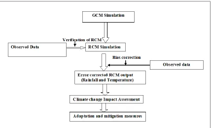
The conceptual model (Fig.2.3) indicates all steps and various relationship that are involved in having confidence with the future climate change projections for local scale impact assessment and development of adaptation strategies. It show the step which this study has adopted from assessment of the temperature and rainfall pattern using observed data, to verification of the model’s output by use of the observed data to finally use of the projections in impact assessment and development of adaptation strategies.
CHAPTER THREE MATERIAL AND METHODS 3.1 Study Area
The area of focus for this study is Kenya. The country is positioned in East Africa. It lies within longitudes 34° E to 42° E, and latitudes 4.5° N to 5° S (Fig. 3.1), with a total area of about 582, 650 km2. Kenya boarders Uganda and Lake Victoria to the west, Somalia to
the east, Tanzania to the south, Ethiopia to the north, Southern Sudan to the North West, and the Indian Ocean to the southeast. The Equator dividing the country into almost two equal parts (Bowden, 2007).
The region has a varied topographical feature, which include the coastal line, Highlands, Lowland, and Great Rift Valley. The relief map of Kenya indicates that quite a large portion of the area lies around 1200 m above mean sea level (AMSL). The highest mountains in Africa are found in this region. These mountains include Mt. Kenya (5199 m), Mt. Kilimanjaro (5895 m), Mt. Elgon (4321 m), Aberdare ranges (3999 m), and Mau Escarpment (3098 m). The study area has large inland water bodies. These include Lakes Victoria, Turkana, Baringo, Naivasha, Nakuru among others. Lake Victoria is the second largest freshwater lake in the world and it generates strong mesoscale circulation in the region.
rivers of the region. The mountains, therefore, form an integral component of the regional hydrological cycle. Certainly, these local factors significantly influence the local circulation pattern and hence the variation of local climate from one place to another.
3.1.1 Climatology of the Study Area
Kenya experiences bimodal rainfall regime, which is locally referred to as 'long rains' season coming in March-May (MAM) and the 'short rains' being reported in October-December (OND) with high amounts mostly reported during the long rain season (Mutai and Ward, 2000; Camberlin and Philippon, 2002; Yang et al., 2015; Ogwang et al., 2015). These rainy seasons coincide with periods of the year when the ITCZ is overhead at the equator (Black et al., 2003; Anyah and Semazzi, 2006). The intervening periods are relatively dry. However, there are rainfall-enhancing mechanisms in the region, which contribute to substantial rains over the western and coastal parts of East Africa in July-August (JJA). These mechanisms include the warm and moist Congo air mass, and the East Africa low-level jet (EALLJ) respectively (Ogallo, 1989).
3.2 Data
Several datasets were used in this study. These are observed daily rainfall and temperature, Monthly gridded rainfall and temperature, Sea surface temperature (SST) and daily Coordinated Downscaled Experiment (CORDEX) dataset for rainfall and temperature (Table 3.1).
Table 3. 1: Summary of the data used in the study
SN Source of Data Type, Period and Resolution Reference 1 Daily observed
station data
Daily mean rainfall, minimum and maximum temperature for 34 stations from 1950 to 2014.
2 Global Precipitation Climatology Centre (GPCC)
Monthly Precipitation data, from 1901 to 2015, at 0.5o by 0.5o resolution
Schneider et al. (2015)
3 Climate Research Units (CRU)
Daily mean maximum and minimum temperature and rainfall from 1901 to 2015, at 0.5o by 0.5o resolution
Harris et al., 2014
University of East Anglia et al. 2014 4 Sea Surface
Temperature
Monthly sea surface temperature from 1960 to 2015 at 1o by 1o resolution
Rayner et al., 2003 5 Coordinated Downscaled Experiment (CORDEX) Africa Datasets
Daily mean rainfall and maximum and minimum temperature, from 1970 to 2100
3.2.1 Observed Station Data
Daily station data for rainfall and temperature for Kenya and extending from January 1950 to December 2014 was obtained from Kenya Meteorological Department (KMD), 33 stations spread across the country were used. The stations were selected based on completeness and quality of data set and spatial distribution over the county (Figure 3.1). The synoptic station that are manned by Kenya Meteorological were mainly used. Other volunteer rainfall station that are available, had missing data more than 20% and had not history of calibration therefore, were not used in this study. The station used, had different length, ranging from 1950 to 2014. The amount of missing data was variable ranging from 4 to 7%. Figure 3.1 shows the spatial distribution of the stations and Table 3.2 gives the name of the station, location in terms of latitude and longitude, elevation of the station and the length of the data.
3.2.2 Gridded Datasets
These datasets refer to the data that incorporate direct observations, remote-sensed data, and modeled data. These data are quality controlled, merged and interpolated at a grid point to obtain gridded dataset. There are different gridded data set from different sources, but for this study, two sets of gridded data were used and they are; Global Precipitation Climatology Centre (GPCC; version 7) and Climate Research Unit (CRU; version TS3.22) spanning from 1901 to 2015.