Binary Overlay on Train of Pulses for Good Correlation Properties

Available online:

https://edupediapublications.org/journals/index.php/IJR/

Binary Overlay on Train of Pulses for Good Correlation Properties

Dharavath Vennela & Dr.S.P. Singh

1

_{Post Graduate scholar, Mahatma Gandhi Institute of Technology, Gandipet, Hyderabad, India.}

2

_{Professor & Head of Department of ECE, Mahatma Gandhi Institute of Technology, Gandipet,}

Hyderabad, India

ABSTRACT

Pulse compression technique is used to achieve high range resolution, but pulse compressor outputs have sidelobes. By overlaying orthogonal binary Phase coding on any coherent train of identical radar pulses can removes most of the autocorrelation near sidelobes and lowers the recurrent lobes.

Keywords: Autocorrelation, Binary codes, pulse Compression, sidelobes

I. INTRODUCTION

Pulse compression codes have used Phase modulation and Frequency modulation. Pulse compression technique is used to achieve high range resolution but pulse compressor outputs have correlation sidelobes. These side lobes can be eliminated to a decent extent by overlaying orthogonal phase coding on any coherent train of identical radar pulses. In this work both binary orthogonal overlay and its Derivative phase (DP) frequency modulation equivalent are discussed.

II. EXPERIMENTAL WORK

There are some signals which are utilized as input signals for project. They are Barker Binary phase coded pulse train, Constant frequency train of pulses, linear frequency modulated pulse train, Costas array of pulse train and modified Costas array of pulse train.

Barker Binary Phase Coded Pulse Train:

The binary phase is represented as the 0 or π for each sub-pulse. The advanced envelope of the phase-coded pulse is given by:

𝑠(𝑡) = 1

√𝑇∑ 𝑠. 𝑟𝑒𝑐𝑡(

𝑡 − (𝑚 − 1)𝑡𝑏

𝑡𝑏 )

𝑀

𝑚=1

Un-modulated or constant frequency pulses:

Before we start considering the train of constant frequency pulses, let us just notice a single pulse first.

The complex envelope of a constant-frequency or un- modulated pulse is given by:

u(t) = 1

√Trect(

t

T )

Radar ambiguity diagram for the signal s(t) is given by

|𝑥(𝜏, 𝑓)|2_{= | ∫ 𝑠(𝑡)𝑠}∗

∞

−∞

(𝑡 − 𝜏)𝑒𝑗2𝜋𝑓𝑡 _𝑑𝑡|2

Where s(t) is input signal. When the target of interest can be located at (τ,f)=(0,0), and the ambiguity diagram is centered at the same point.

Solving the integrals and taking absolute value provides,

|𝑥(𝜏, 𝑓)|2_{= | (1 −}|𝜏|

𝑇)

sin[𝜋𝑇𝑓(1−|𝜏|

𝑇)]

𝜋𝑇𝑓(1−|𝜏|

𝑇)

| , |τ|≤T,

Zero elsewhere the cut along the delay axis is obtained by setting f=0, providing

|x (τ,0)|2 _{= 1 −}|τ|

T , |τ|≤T, Zero elsewhere

The cut along the Doppler axis is obtained by setting τ=0, providing

|x (0, f)|2 _{= |}sinπfT

πfT |

Linear Frequency Modulated Pulse Train:

Available online:

https://edupediapublications.org/journals/index.php/IJR/

The advanced envelope of a linear-FM pulse is given by

𝑠(𝑡) = 1

√𝑇𝑟𝑒𝑐𝑡(

𝑡

𝑇)exp (𝑗𝜋𝜋𝑘𝑡) , k=±B/T

Costas Array of Pulse Train:

Costas used frequency coding as the alternative of the linear law utilized in LFM. The distinction is incontestable by the binary matrices in Fig. 1. The columns represent M contiguous time slices (each of period tb), and therefore the rows represent M

distinct frequencies, equally spaced by ∆f

Binary matrix of linear frequency modulated and Costas coding

The frequency hopping orders represented in Fig.1 are solely two out of M! Possible orders that meet the restriction of one dot per column and per row. The hopping order powerfully affects the ambiguity function (AF) of the signal. The AF may be expected roughly by overlaying a replica of the binary matrix on itself, so shifting one relative to the opposite consistent with the specified delay (horizontal shifts) and Doppler (vertical shifts). Once a given delay–Doppler shift leads to a coincidence of N points, the ambiguity function is expected to provide a peak of roughly N/M at the corresponding delay–Doppler coordinate.

OVERLAYING CODES

Orthogonal Phase Overlay Matrix:

The orthogonal set was enforced using phase modulation. Associate example of a P-by-M binary orthogonal set, wherever P =M =8, may be delineate with the phase matrix [1],

The actual orthogonal set is given by the matrix

A={ap,m}={exp(jᵠp,m)}

Clearly, the elements of A get solely two values: +1 and -1. Recall that the matrix A is alleged to be orthogonal once the real number between any two columns of A is zero, implying that the matrix

AT_{A is diagonal. Note additionally that orthogonal}

P-by-M matrices A exist just for M · P. The overlay is enforced by phase modulating the pth pulse by the pth row of A. One downside caused by adding a binary phase-coded overlay, is that the broadening of the spectrum.

Derivative Phase (DP) Overlay Matrix:

DP modulation differs from standard binary phase modulation by replacement phase jumps with phase slopes [1]. The frequency steps area unit therefore designed that at the end of the slice period ts the accumulated phase change is that the desired

zero or𝜋. Phase accumulation of π (or -π) is achieved by maintaining the frequency step of -∆f throughout the complete slice. The DP used here is the split slice, within which the frequency modulation (FM) is [∆f,-∆f] is utilized in the primary slice of a sequence, and whenever this slice is a twin of the previous slice [-∆f,-∆f] is employed once this slice is totally different from the previous slice.

Available online:

https://edupediapublications.org/journals/index.php/IJR/

III. RESULTS AND DISCUSSION

For Un-Modulated Pulses

With no overlay: As we can observe that the ambiguity function obtained from this input is called BED of NAILS.

The coherent pulse train provides independent control of delay and Doppler resolutions that is not possible in single pulse case. The delay resolution is controlled by pulse duration while the Doppler resolution is controlled by the total signal length. On the other hand the Doppler and delay ambiguities are tied. We can observe that there are many side lobes in the AF of un-modulated pulse train. These side lobes can be reduced by overlaying methods.

Signal structure of un-modulated pulses with no overlay.

ACF of un-modulated pulses with no overlay.

Ambiguity function of un-modulated pulses with no overlay

With orthogonal phase overlay: The actual orthogonal set is given by the matrix A={ap,m}={exp(jᵠp,m)}. A train of eight constant

frequency (i.e., un-modulated) pulses, with and without binary overlay. Figs.3 (a), 3(b), and 3(c) present the signal structure, ACF, and ambiguity function of a coherent train of un-modulated pulses. Therefore it is aforementioned orthogonal phase overlaying decreases side-lobes however it broadens the spectrum.

Signal structure of constant frequency pulses with orthogonal phase overlay.

0 50 100 150 200 250 300 350

0 0.5 1

A

m

p

lit

u

d

e

0 50 100 150 200 250 300 350

0 0.5 1

P

h

a

s

e

[

ra

d

]

0 50 100 150 200 250 300 350

0 0.5 1

t / t_b

f

*

M

tb

0 10 20 30 40 50 60 70

-90 -80 -70 -60 -50 -40 -30 -20 -10 0

/t_b

A

u

to

c

o

re

la

ti

o

n

[

d

B

]

Autocorrelation function of un-modulated pulses with no overlay

-100 0

100

0 1 2 3 4 5 0 0.5 1

 /t_b

Ambiguity function of unmodulated pulses with no overlay

 *Nt b

|



(



,



)|

0 50 100 150 200 250 300 350 0

0.5 1

A

m

p

li

tu

d

e

0 50 100 150 200 250 300 350 0

1 2 3

P

h

a

s

e

[

ra

d

]

0 50 100 150 200 250 300 350 -100

0 100

t / t_b

f

*

M

Available online:

https://edupediapublications.org/journals/index.php/IJR/

ACF of constant frequency pulses with orthogonal phase overlay.

Ambiguity function of constant frequency pulses with orthogonal phase overlay.

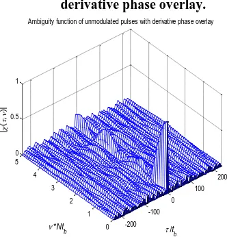
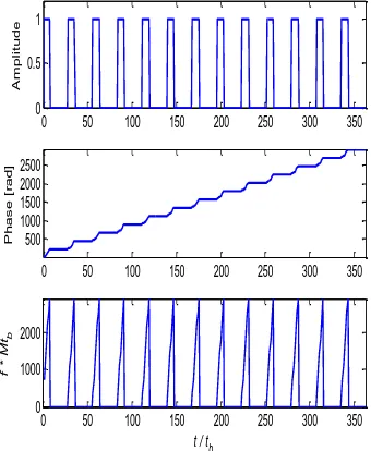
With derivative phase overlay: Fig 4(a) shows the ACF of un-modulated pulses with derivative phase overlays shown in fig spectrums of the complicated envelope of the signal are going to be shifted downward in frequency. Fig 4(b) shows the Ambiguity function of constant frequency pulses with derivative phase overlay.

ACF of constant frequency pulses with

derivative phase overlay.

Ambiguity function of constant frequency pulses with derivative phase overlay. Pulse train with 13 bits Barker Codes

By overlaying the orthogonal phase matrix on barker phase modulated input the side-lobes is reduced to a good extent and also the derivative phase overlaying is additional economical in removal of side-lobes. Fig 5(a) shows the Signal structure of barker code of 13 elements with no overlay. Fig 5(b) shows the Ambiguity function of barker code with no overlay. Fig 5(c) shows the Ambiguity function of barker code with orthogonal phase overlay. Figure 5(d) shows the Ambiguity function of barker code with derivative phase overlay. It shows that so most of the close to side lobes area unit removed.

Signal structure of barker code of 13 elements with no overlay.

0 10 20 30 40 50 60 70

-90 -80 -70 -60 -50 -40 -30 -20 -10 0

/tb

A

u

to

c

o

re

la

ti

o

n

[

d

B

]

Autocorrelation function of unmodulated pulses with orthogonal phase overlay

-100 0

100

0 1 2 3 4 5 0 0.5 1

 /t

b Ambiguity function of unmodulated pulses with orthogonal phase overlay

 *Nt

b

| ( ,

)|

0 10 20 30 40 50 60 70 80 90

-90 -80 -70 -60 -50 -40 -30 -20 -10 0

/t_b

A

u

to

c

o

re

la

ti

o

n

[

d

B

]

Autocorrelation function of unmodulated pulses with derivative phase overlay

-200 -100

0 100

200

0 1 2 3 4 5 0 0.5 1

 /t_b

Ambiguity function of unmodulated pulses with derivative phase overlay

 *Nt

b

|



(



,



)|

0 50 100 150 200 250 300 350 0

0.5 1

A

m

p

li

tu

d

e

0 50 100 150 200 250 300 350 0

1 2 3

P

h

a

s

e

[

ra

d

]

0 50 100 150 200 250 300 350 -100

0 100

t / t_b

f

*

M

Available online:

https://edupediapublications.org/journals/index.php/IJR/

Ambiguity function of barker code with no overlay.

Ambiguity function of barker code with orthogonal phase overlay.

Ambiguity function of Barker code with derivative phase overlay.

For LFM of pulse train

In this case pulse in pulse train has linearly increasing frequency. Fig 6(a) shows the Signal structure of LFM pulses. Fig 6(b) shows the Ambiguity function of LFM pulses with no overlay. Fig 6(c) shows the Ambiguity function of LFM pulses with orthogonal phase overlay. Fig 6(d) shows the Ambiguity function of LFM pulses with derivative phase overlay.

Signal structure of LFM pulses.

Ambiguity function of LFM pulses with no overlay.

-200 0

200

0 1 2 3 4 0 0.5 1

 /t_b

Ambiguity function of barker code of 13 elements with no overlay

 *Nt_b |

( ,

)|

-200 0

200

0 1 2 3 4 0 0.5 1

 /t

b

Ambiguity function of barker code of 13 elements with orthogonal phase overlay

 *Nt_b

| ( ,

)|

-400 -200

0 200

400

0 1 2 3 4 0 0.5 1

 /t b

Ambiguity function of barker code of 13 elements with derivative phase overlay

 *Nt b

| ( ,

)|

0 50 100 150 200 250 300 350

0 0.5 1

A

m

p

li

t

u

d

e

0 50 100 150 200 250 300 350

500 1000 1500 2000 2500

P

h

a

s

e

[

r

a

d

]

0 50 100 150 200 250 300 350

0 1000 2000

t / t_b

f

*

M

tb

-200 0

200

0 1 2 3 4 0 0.5 1

 /t_b

Ambiguity function of LFM pulses with no overlay

 *Nt_b

| ( ,

Available online:

https://edupediapublications.org/journals/index.php/IJR/

Ambiguity function of LFM pulses with orthogonal phase overlay.

Ambiguity function of LFM pulses with derivative phase overlay.

IV. CONCLUSION

In this work binary phase orthogonal overlay and derivative phase overlay on Barker coded pulse train and linear frequency coded pulse train signal is discussed. It is found that overlay coding deceases autocorrelation side-lobe.

V. REFERENCES

[1] Nadav Levanon “Implementing Orthogonal Binary Overlay on a Pulse Train using Frequency Modulation” IEEE Transactions on aerospace and electronic systems vol. 41, no. 1 January 2005

[2] Radar Signals by Nadav Levanon and Eli Mozeson.

[3] International radar symposium India- 2005.

[4] Merill I. Skolinik, “Introduction to Radar System”, Tata McGraw Hill publications Third edition, 2001.

[5] Byron Edde, “Radar principles, Technology Applications”, Prientice Hall publications, 1993.

-200 0

200

0 1 2 3 4 0 0.5 1

 /t_b

Ambiguity function of LFM pulses with orthogonal phase overlay

 *Nt_b

|



(



,



)|

-400 -200

0 200

400

0 1 2 3 4 0 0.5 1

 /t b Ambiguity function of LFM pulses with derivative phase overlay

 *Nt b

|



(



,

