A New Method to Solve Same-different Problems with Few-shot Learning

(1)

Western University Western University

Scholarship@Western

Electronic Thesis and Dissertation Repository

12-4-2019 3:30 PM

A New Method to Solve Same-different Problems with Few-shot

Learning

Yuanyuan Han

The University of Western Ontario

Supervisor Charles Ling

The University of Western Ontario Graduate Program in Computer Science

A thesis submitted in partial fulfillment of the requirements for the degree in Master of Science © Yuanyuan Han 2019

Follow this and additional works at: https://ir.lib.uwo.ca/etd

Part of the Other Computer Sciences Commons

Recommended Citation Recommended Citation

Han, Yuanyuan, "A New Method to Solve Same-different Problems with Few-shot Learning" (2019). Electronic Thesis and Dissertation Repository. 6716.

https://ir.lib.uwo.ca/etd/6716

This Dissertation/Thesis is brought to you for free and open access by Scholarship@Western. It has been accepted for inclusion in Electronic Thesis and Dissertation Repository by an authorized administrator of

(2)

Abstract

Visual learning of highly abstract concepts is often simple for humans but very challenging

for machines. Same-different (SD) problems are a visual reasoning task with highly abstract

concepts. Previous work has shown that SD problems are difficult to solve with standard deep

learning algorithms, especially in the few-shot case, despite the ability of such algorithms to

learn abstract features. In this paper, we propose a new method to solve SD problems with

few training samples, in which same-different visual concepts can be recognized by

exam-ining similarities between Regions of Interest by using a same-different twins network. Our

method achieves state-of-the-art results on the Synthetic Visual Reasoning Test SD tasks and

outperforms several strong baselines, achieving accuracy above 95% on several tasks and above

85% on average with only 10 training samples. On a few of these challenging SD tasks, our

approach even outperforms reported human performance [30]. We further evaluate the

per-formance of our method outside of the synthetic tasks and achieve good perper-formance on the

MNIST, FashionMNIST and Face Recognition datasets.

Keywords: Few-shot Learning, Deep Learning, Same-Different, Regions of Interest

(3)

Summary for Lay Audience

In recent years, computer vision has witnessed many significant breakthroughs in standard

recognition tasks such as image classification, image segmentation, or object detection. Most

of these gains are a result of applying deep convolutional neural networks (CNNs). However,

visual learning tasks requiring attention to highly abstract concepts such as ”sameness” and

”difference” have proven especially difficult for standard deep CNNs, although it may be

sim-ple and obvious for humans. The ability to recognize visual tasks with highly abstract concepts

is a ubiquitous human skill that has not seen significant progress for the machine.

Besides, humans can learn these highly abstract visual concepts such as ”sameness” and

”difference” with little supervision. When one person only met someone once, he can

remem-ber who they are when he meets them on the street next time. In this thesis, we primarily deal

with the same-different classification through few-shot learning. In particular, we try to solve

SVRT same-different visual reasoning problems by using few-shot learning and then apply our

model to solve more complex same-different problems in real life.

(4)

Acknowlegements

To my supervisor, Dr. Charles Ling, I owe an immense debt of gratitude for his support,

men-torship, scientific insights and contagious enthusiasm during my studies. His consistent, patient

confidence in me was essential in the performance of the work described in this thesis. He

pro-vides much help since I came to Canada, I believe he considerably exceeded the expectations

of his role as supervisor.

I would like to thank Xuezhi, Yining, Xinxu and Tanner for their encouragement and

ad-vices during this research and the life in Canada.

I would also like to show special gratitude to my parents for their constant support

through-out my research and life.

(5)

List of Figures

1.1 The image in (a) can be classified as containing the car by CNNs with high

confidence. However, CNN fails to learn the concept of “sameness” and

“dif-ference”: the first image in (b) has two different curves and the second image

in (b) has two same curves. The image in (b) is from the Synthetic Visual

Reasoning Test tasks [10]. . . 2

1.2 A few same-different examples from the SVRT tasks. . . 4

1.3 A few “sameness” examples generated by MNIST, Fashion-MNIST,

miniIm-agenet and Face datasets. The first line of images needs to deal with fuzzy

“sameness” and the second line needs to solve visual reasoning. In second line,

(a) contains one exact duplicate. (b) contains one fuzzy duplicate. (c)

con-tains one exact duplicate with some transformations (scaling and rotating). (d)

contains one fuzzy duplicate with some transformations . . . 6

2.1 Examples for several abstract visual reasoning tasks . . . 9

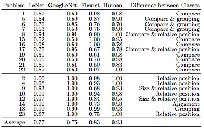
2.2 Completed experimental results with humans (taken from the source:

Compar-ing machines and humans on a visual categorization test, Fleuret et al. [10]).

Each row corresponds to one of the 23 problems and each column to one of the

20 participants. Each cell contains the number of attempts before seven

con-secutive correct categorizations were made. Entries containing “X” indicate

that the participant failed to solve the problem, and those cells are not included

in the marginal means [10]. . . 10

(9)

2.3 Experiment results on the SVRT classification tasks (taken from the source: 25

years of cnns: Can we compare to human abstraction capabilities?, Stabinger

et al. [30]) . . . 11

2.4 General strategy for siames neural network(taken from the source: Siamese

neural networks for one-shot image recognition, Koch et al. [18]). . . 12

2.5 A sample 2 hidden layer siamese network for binary classification with logistic

prediction p (taken from the source: Siamese neural networks for one-shot

image recognition, Koch et al. [18]). . . 13

2.6 An example for meta-learning (learn to learn) based few-shot learning method. 14

2.7 Matching Networks architecture(taken from the source: Matching networks for

one shot learning, Vinyals et al. [34]) . . . 16

2.8 Prototypical Networks in the few-shot and zero-shot (no labeled example)

sce-narios (taken from the source: Prototypical networks for few-shot learning,

Jake Snell et al. [29]). . . 17

2.9 Relation Network architecture for a 5-way 1-shot problem with one query

ex-ample (taken from the source: Learning to compare: Relation network for

few-shot learning, Flood Sung et al. [31]). . . 18

3.1 A few samples in “sameness” class for SVRT #1 . . . 21

3.2 The simplified process in solving the SVRT SD problems through our approach 22

3.3 The method of calculating IoU in the field of image . . . 23

3.4 Convolutional architecture for the embedding module . . . 25

3.5 Relation module for few-shot learning SD problems . . . 26

4.1 The Omniglot dataset contains different images from alphabets across the world. 30

4.2 A few samples of random data augmentation generated for three images in the

Omniglot data set . . . 31

(10)

4.3 Examples of the fifth-layer convolutional filters learned by same-different twins

network. . . 36

5.1 Generalize to evaluate 10-way one-shot task on MNIST based on learned fea-tures from Omniglot . . . 41

5.2 A few examples for MNIST same-different visual reasoning tasks . . . 42

5.3 Generalize to evaluate 10-way one-shot task on Fashion-MNIST based on learned features . . . 44

5.4 A few examples from Fashion-MNIST SD visual reasoning tasks . . . 45

5.5 A sample for the generated pairs using AT&T Database of Faces . . . 47

5.6 One-shot task on facial recognition . . . 48

A.1 Summary for Same-different Twins Network (input size: 84 x84) . . . 58

A.2 Summary for Same-different Twins Network (input size: 28 x28) . . . 59

B.1 Summary for Fine-tune deep CNNs (Vgg-16) . . . 61

B.2 Summary for Model-Agnostic Meta-Learning . . . 62

B.3 Summary for Prototypical Network . . . 63

B.4 Summary for Relation Network . . . 64

B.5 Summary for Convolutional Siamese Network . . . 65

(11)

List of Tables

4.1 Comparing the one-shot accuracy between the Siamese network and

Same-different twins network. . . 36

4.2 A summary of the test results on the SVRT SD problems for different methods. 38 5.1 Experiment results for MNIST 10-way one-shot classification tasks. . . 42

5.2 Experiment results for MNIST same-different visual reasoning tasks. . . 43

5.3 Results for Fashion-MNIST 10-way one-shot classification task. . . 45

5.4 Experiment results for FashionMNIST SD visual reasoning tasks. . . 46

5.5 Experiment results for one-shot facial recognition task. . . 48

(12)

Chapter 1 Introduction

In this chapter, we provide some background on same-different problems and discuss the

im-portance of the research question and our contribution toward solving it. The thesis layout is

introduced at the end.

1.1 Background

In recent years, computer vision has witnessed many significant breakthroughs in standard

recognition tasks such as image classification [19], image segmentation [6] (the process of

par-titioning a digital image into multiple segments) or object detection [26]. Most of these gains

are a result of applying deep convolutional neural networks (CNNs). However, visual learning

tasks requiring attention to highly abstract concepts such as “sameness” and “difference” have

proven especially difficult for standard deep CNNs [30,17].

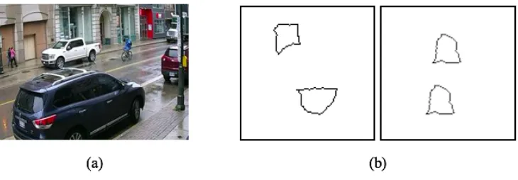
Considering the two images in Figure 1.1, the image on the left (a) could have been

cor-rectly classified as containing the cars by the deep convolutional neural network after the

net-work was trained on thousands of images. However, similar algorithms struggle to learn the

concepts of “sameness” and “difference” for the image on the right (b) even after seeing

mil-lions of training examples, although it may be simple and obvious for humans. The ability to

recognize visual tasks with highly abstract concepts is a ubiquitous human skill that has not

(13)

2 Chapter1. Introduction

Figure 1.1: The image in (a) can be classified as containing the car by CNNs with high con-fidence. However, CNN fails to learn the concept of “sameness” and “difference”: the first image in (b) has two different curves and the second image in (b) has two same curves. The image in (b) is from the Synthetic Visual Reasoning Test tasks [10].

seen significant progress for the machine.

The study of same-different problems has many practical implications. One of the popular

applications is face similarity recognition [15]. Face recognition can help us verify identity or

do some face analysis. In modern mobile devices, there are many features developed based

on face recognition, such as the ability to turn on our phone or open our bank app via face

recognition. Face recognition can also help us target people from many people. The research

of same-different problems can significantly improve the performance of face recognition.

Besides, humans can learn these highly abstract visual concepts such as “sameness” and

“difference” with little supervision. When a person meets someone once, they can usually

remember who the person is when they meet on the street next time. In the Synthetic Visual

Reasoning Test tasks (SVRT) [10], it has also been proven that humans can learn the concepts

of “sameness” and “difference” with only few examples [30, 10]. However, for most deep

learning models, they need large amounts of labeled training data to train their large number

of parameters. Considering that (1) there aren’t many labeled dataset in real life and much

annotation is needed for new classes which is very time-consuming and labor-intensive, (2) in

some cases, numerous annotated images may simply never exist for newly emerging categories

(14)

1.2. ResearchQuestion 3

essential and helpful.

All these motivate the study we are interested in: few-shot learning same-different tasks,

which aims to recognize “sameness” and “difference” visual categories based on very few

labeled examples. It would be a huge challenge to solve the same-different problems due to

that: (1) Previous work shows that standard deep learning methods are not capable of solving

same-different problems even when provided with millions of training samples [30, 17]. (2)

The availability of only one or very few examples challenges the standard ‘fine-tuning’ practice

in deep learning [9] and more easily causes over-fitting.

1.2 Research Question

In this thesis, we primarily deal with the same-different classification through few-shot

learn-ing. In particular, we try to solve SVRT same-different problems by using few-shot learning

and then apply our model to solve more complex same-different problems in real life.

1.2.1 SVRT Visual Reasoning Tasks

Synthetic Visual Reasoning Test tasks include 23 tasks. The 23 SVRT tasks can be split into

two groups based on the type of patterns: spatial relation (SR) problems (ex. shapes in a line vs.

not in a line) and same-different (SD) problems (ex. two pairs of unique shapes vs. two pairs of

identical shapes) [30]. Previous attempts on SVRT problems show deep learning approaches

are capable of solving SR problems, at least when provided with plenty of training data (20K

training images in [30] and 1 million used in [17]), but fail to solve SD problems even when

provided with millions of training samples [30,17].

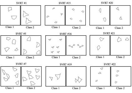
A few examples of SD problems taken from the SVRT tasks are given in Figure 1.2. Each

pair of images stands for one SVRT task, and the pair is divided into two classes: “sameness”

(Class2) and “difference” (Class1). In the “sameness” class, in addition to determining

(15)

Figure 1.2: A few same-different examples from the SVRT tasks.

and “invariant on scaling and rotating” are also included. Therefore, we not only need to deal

with “sameness” and “difference”, but also need to solve the visual reasoning based on

“same-ness” and “difference”. Some same-different problems in the SVRT tasks are even very difficult

for human beings such as SVRT #5, #7, #16, #21 [10]. These tasks need to deal with some

highly abstract visual reasoning such as“grouping”, “reflection”, and “invariant on scaling and

rotating”.

For SVRT #5, both classes contain four random objects. Class 1 contains four different

objects, while class 2 contains two pairs of the same objects. For SVRT #7, both classes

contain six objects. In class 1, objects can be organized into three groups, each containing

two same objects. In class 2, objects can be organized into two groups, each consisting of

three same objects. SVRT #16 requires the agent to decide whether shapes on the right side

(16)

1.3. Contributions 5

very challenging task. Each image contains two objects. One of the objects in class 2 can be

obtained from the other by scaling, translating, and rotating.

Francois Fleuret et al. studied SVRT tasks. In their experiment of few-shot learning for

SVRT SD problems, the prediction accuracy remained virtually at 50% for every problem [10].

Many SD tasks only have about 50% accuracy, even trained by plenty of training samples [30].

So it would be a huge challenge to solve the same-different problems with few training samples.

In this thesis, we will study how to use few training samples to determine whether two objects

the same or different and how to make visual reasoning based on “sameness” and “difference”,

so as to correctly classify the new image into its category.

1.2.2 Other Same-di

ff

erent Problems

We also apply our model to solve more other SD problems in real life. These problems are

gen-erated through other datasets such as MNIST, Fashion-MNIST, and Face datasets, and need to

deal with some fuzzy “sameness” and visual reasoning based on “sameness” and “difference”.

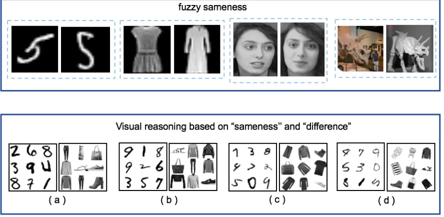
Figure 1.3 shows several “sameness” examples for these same-different problems. Chapter 5

introduces these problems in detail and shows how we solve them by using our model. Through

these applications, it has been shown that our model can be used in a wider variety of

same-different problems.

1.3 Contributions

In this thesis, we proposed a new method to solve SD visual classification problems when a

few training samples are provided. Our new approach is inspired by research on object

de-tection and few-shot learning. This method is divided into three parts: (1) Regions of Interest

(RoIs) are obtained through selective search method; (2) Similarities between RoIs are learned

through the same-different twins network. (3) The class labels for new images are recognized

(17)

Figure 1.3: A few “sameness” examples generated by MNIST, Fashion-MNIST, miniImagenet and Face datasets. The first line of images needs to deal with fuzzy “sameness” and the second line needs to solve visual reasoning. In second line, (a) contains one exact duplicate. (b) con-tains one fuzzy duplicate. (c) concon-tains one exact duplicate with some transformations (scaling and rotating). (d) contains one fuzzy duplicate with some transformations

abstract visual reasoning of “sameness” and ”difference” into the problem of calculating the

similarities between the Regions of Interest. Therefore, the classification tasks of “sameness”

and “difference” can be solved more directly and efficiently. By using the region comparison

methods, we are able to achieve accuracies above 90% on several tasks and above 85% on

av-erage with only ten training samples. Our method even surpasses reported human performance

on some SD tasks such as SVRT #5, #15, and #16 [10]. We also evaluate the performance of

our approach on other SD tasks generated by using MNIST, Fashion-MNIST, and face dataset.

These tasks need to deal with some fuzzy “sameness” and our method also achieves good

performance on these tasks.

The main contribution of this thesis is as following:

• We developed a same-different twins network that can be used to solve the same-different

(18)

1.4. Structure of thisThesis 7

3.2.2.

• We built a novel model to solve SVRT SD problems with few-shot learning through

com-bining regions of interest module, same-different twins network, and pattern recognition

module together, achieving state-of-the-art performance on all SVRT SD problems,

see-ing Chapter 3.

• We benchmarked several popular few-shot learning algorithms on the SVRT SD

prob-lems and demonstrated the strength of our approach on few-shot learning of SD visual

tasks, outperforming the previous state-of-the-art as well as several strong baselines,

seeing Chapter 4. We believe this work will inspire future development in solving the

same-different problems.

• We evaluated the performance of our method on several other SD tasks generated by

using MNIST, Fashion-MNIST, and Face dataset, showing that our method could be

applied to a broader variety of same-different problems, seeing Chapter 5.

1.4 Structure of this Thesis

This thesis aims to solve the same-different problems through few-shot learning. This Chapter

has introduced the background and the research problems in this thesis. The rest of the thesis

is organized as follows. In Chapter 2, we provide an overview of the related work, including

research on SD visual reasoning tasks and few-shot learning methods and Regions of Interest

selection. In Chapter 3, we describe our new approach to solving the same-different visual

reasoning problems. In Chapter 4, we discuss the experiments, including the datasets that we

use, baseline models, and experiment results. In Chapter 5, we use our model to solve more

other SD tasks generated through other datasets such as MNIST, Fashion-MNIST, and Face

(19)

Chapter 2 Related Work

In this chapter, we will briefly review the previous work done on same-different problems,

describe various few-shot learning methods in image classification, and provide an overview

of approaches for selection of Regions of Interest.

2.1 Research on Same-di

ff

erent Problems

Same-different problems contain standard same-different classification tasks (whether two

im-ages belong to the same category) in a broad sense and same-different visual reasoning task

(some highly abstract visual concepts are contained in one image).

2.1.1 Same-di

ff

erent Visual Reasoning Tasks

There are several potential sources of abstract visual reasoning tasks. These embody the

CLEVER dataset (answer queries based on a scene with multiple objects) [16], Bongard

prob-lems (classify the new images through seeing six labeled pictures in each class) [4], Raven’s

Progressive Matrices (given several patterns, identify the missing pattern) [24], and Synthetic

Visual Reasoning Test tasks (SVRT) (given N labeled images, classify unseen new images) [10].

Figure 2.1 shows several examples of these abstract visual reasoning tasks. Unlike Ravens

(20)

2.1. Research onSame-differentProblems 9

Figure 2.1: Examples for several abstract visual reasoning tasks

gressive Matrices and CLEVR datasets that have seen significant progress [2,14], SVRT tasks

and Bongard problems only have seen partial success. SVRT tasks can be divided into two

kinds of tasks: spatial relation tasks and same-different visual reasoning tasks. Perhaps due

to the difficulty in learning to solve same-different problems in SVRT tasks, most work in this

same-different visual reasoning task has focused on examining how and why machine learning

approaches have failed.

Francois Fleuret et al. [10] first introduced the SVRT tasks and showed that humans are

much more proficient at these tasks than the presented machine learning approaches. They

used SVRT tasks to compare the efficiency in binary image classification between human and

machine learning and demonstrated that the SVRT tasks were easy to spot and characterize

for humans, but those tasks were challenging to learn for generic machine learning systems.

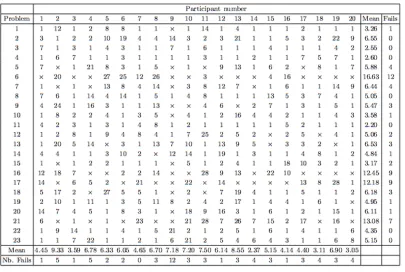
Figure 2.2 shows the human performance on SVRT tasks tested by Fleuret et al [10]. 20 people

who participated in Fleuret’s experiments would be randomly given one image from the two

(21)

10 Chapter2. RelatedWork

Figure 2.2: Completed experimental results with humans (taken from the source: Comparing machines and humans on a visual categorization test, Fleuret et al. [10]). Each row corresponds to one of the 23 problems and each column to one of the 20 participants. Each cell contains the number of attempts before seven consecutive correct categorizations were made. Entries containing “X” indicate that the participant failed to solve the problem, and those cells are not included in the marginal means [10].

correctly identified the class 7 times in a row, it proved that he/she learned this rule, and when

35 consecutive failures occurred to the classification, it proved that he/she failed to learn the

rule.

For machine learning methods, Fleuret et al. [10] paired three different feature groups with

two classification algorithms, and found that the best performing pair combined Fourier and

wavelet coefficients derived from the images with Adaboost [11]. However, in their few-shot

experiments (with only ten labeled examples of each problem), the performance on most of

the 23 tasks was roughly random, with accuracy about 50%. With a large number of training

samples, the difficulty between same-different and spatial relation tasks became more

(22)

Figure 2.3: Experiment results on the SVRT classification tasks (taken from the source: 25 years of cnns: Can we compare to human abstraction capabilities?, Stabinger et al. [30])

on average on same-different tasks and 88% accuracy on average on spatial relation tasks.

Some same-different problems could not be solved with even 10,000 training examples with a

performance of around 60%.

A unique approach to solving SVRT tasks is presented by Kevin Ellis et al. [7]. They

introduced an unsupervised learning algorithm to solve SVRT tasks. Their method synthesized

programs from data. First, their model parsed the images into symbolic forms by locating

distinct shapes (SVRT tasks are particularly amenable to this). Then, using a grammar tuned for

the task, their algorithm searched over a space of drawing programs, looking for those that best

reproduce the original image over the space. Once a program had been found for each training

image, a classifier was trained to map drawing programs to class labels, where it demonstrated

strong performance. The algorithm could learn how abstract structures are represented in vision

and achieve excellent performance on SVRT tasks. However, this approach is quite slow, and

some images may take hundreds of seconds to synthesize the program.

When studying the SVRT problems with more modern computer vision approaches,

(23)

Figure 2.4: General strategy for siames neural network(taken from the source: Siamese neural networks for one-shot image recognition, Koch et al. [18]).

and GoogLeNet [32] CNNS. Figure 2.3 shows the experimental results on the SVRT

classifi-cation tasks from Stabinger et al. They found that near-perfect performance was achievable on

roughly half of the tasks, with the other half being significantly more difficult (near-random).

By observing the abstract concepts required to solve each SVRT task, they noticed that the

easy-difficult split closely corresponded to whether or not tasks required same-different

com-parisons, with a couple of exceptions (they determined that a couple of same-different problems

could be solved by exploiting simple pixel distribution patterns). The authors found that both

CNNs perform very similarly, working well on spatial relation problems and not seem to have

made much progress on same-different problems, despite training each network on 20,000

im-ages per class. Many same-different tasks only achieved about 50% accuracy even when CNNs

were trained by plenty of training sets. The general inability for CNNs to learn to solve SD

tasks is also supported by [17], where a more systematic examination of the performance of an

(24)

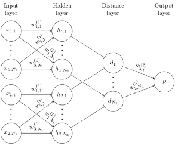
Figure 2.5: A sample 2 hidden layer siamese network for binary classification with logistic prediction p(taken from the source: Siamese neural networks for one-shot image recognition, Koch et al. [18]).

2.1.2 Standard Same-di

ff

erent Classification Tasks

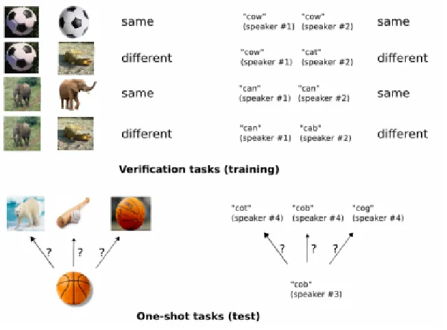
Koch et al. [18] built a Convolutional Siamese Neural Network to solve same-different image

recognition problems by one-shot learning. Figure 2.4 shows the general strategy for Siamese

Neural Network. The author first trained a model to discriminate between a collection of

same/different pairs, and then made the model generalize to evaluate new categories based

on learned feature mappings for verification. A Siamese Neural Network consists of twin

networks that accept distinct inputs but are joined by an energy function at the top. This

function computes some metric between the highest-level feature representation on each side,

as shown in Figure 2.5. In this thesis, we developed our same-different twins network based

on the Siamese Neural Network by changing the feature embedding layer and distance metric

(25)

Figure 2.6: An example for meta-learning (learn to learn) based few-shot learning method.

2.2 Few-shot Learning Methods

The study of few-shot learning has become a hot research direction for some time. Few-shot

classification [22,20,18] is a task in which a classifier must be trained to recognize new classes

not seen in the training samples when few training examples are given. A simple method, such

as re-training the model on the new training samples, would lead to severe over-fitting. While

the problem is quite tricky for the machine, it is straightforward for human beings. It has

been demonstrated that humans can perform even one-shot classification where only a single

example of each new class is given with high accuracy [20].

Earlier work on few-shot learning mainly introduced generative models by using some

complex strategies such as probabilistic models based on the Bayesian approach [8,20]. With

the success of deep learning on large-scale data sets [19,12, 28], many people contributed to

generalizing deep learning-based approaches to solve few-shot learning problems. Many of

those approaches use a meta-learning or learning-to-learn strategy, which means that they

ex-tract some transferable knowledge from previous tasks or some auxiliary tasks, such as

transfer-learning method. This transferable knowledge can help to learn the target few-shot problems

well without suffering from the over-fitting that often occurs when applying deep learning

(26)

2.2. Few-shotLearningMethods 15

Meta-learning can be divided into two phases: meta-training phase and meta-test phase. In

the meta-training phase, the training data sets are decomposed into different meta tasks, which

help the model to learn the generalization ability in the case of category change. If a meta-task

containsCdistinct classes andKexamples in each class, the target few-shot problem is called

C-wayK-shot. In the meta-test phase, classification for the new class can be completed without

changing the existing model. Figure 2.6 shows an example for meta-learning (learn to learn)

based few-shot learning method. There are mainly three kinds of meta-learning models in

modern few-shot learning methods: Fine-Tune based, RNN based, and Embedding and Metric

Learning based.

2.2.1 Few-shot Learning based on Fine-Tuning

Deep CNNs have recently shown outstanding image classification performance in large-scale

visual recognition challenges. However, to train a CNN requires a large number of labeled

image samples because CNN has millions of parameters that need to be estimated. For

few-shot learning tasks, it is obviously not feasible. A solution is to use a pre-trained CNN as a

feature extractor [23]. Transfer Learning is the reuse of a pre-trained model on a new problem.

When solving a new problem, most of the layers in front of the model are frozen, and we only

need to fine-tune the last few layers. It is currently popular in the field of deep learning because

it enables us to train deep neural networks with comparatively little data.

C. Finn et al. [9] proposed Model-Agnostic Meta-Learning (MAML) approach, which

aimed to train a given neural network model on a variety of learning tasks to obtain the initial

weight configuration, such that it can solve new tasks using only few training samples. The

strategy here is to meta-learn an initial set of neural network weights (the parameters of the

model), so the neural network models can be effectively fine-tuned to produce excellent

gener-alization performance on the new few-shot learning tasks within few gradient-descent update

steps. S Ravi et al. [25] further proposed the few-shot optimization method, which used an

(27)

net-16 Chapter2. RelatedWork

Figure 2.7: Matching Networks architecture(taken from the source: Matching networks for one shot learning, Vinyals et al. [34])

.

work weights but an LSTM-based optimizer. The optimizer can be trained to be specifically

effective for fine-tuning. The biggest problem for the fine-tune based meta-learning methods is

that these approaches need to fine-tune on the target problems.

2.2.2 Few-shot Learning based on RNN Memory

Adam Santoro et al. proposed meta-learning with memory-augmented neural (MANN)

net-works [27] that uses recurrent neural networks (RNN) with memories. Meta-learning means

that the weights of the RNN are trained by learning many distinct meta tasks. The strategy

here is to use RNN to accumulate the knowledge in its hidden activations or external memory

through iterating on the meta-training examples. The stored knowledge can help to solve the

target few-shot problems. When classifying new classes, it can be done by comparing them

with historical information stored in the memory. The main challenge for MANN is to

en-sure that all the relevant historical information has been reliably stored in the RNN without

(28)

2.2. Few-shotLearningMethods 17

Figure 2.8: Prototypical Networks in the few-shot and zero-shot (no labeled example) scenarios (taken from the source: Prototypical networks for few-shot learning, Jake Snell et al. [29]).

2.2.3 Few-shot Learning based on Embedding and Metric Learning

Another kind of popular meta-learning based few-shot learning method is the embedding and

metric learning approach. This method aims to learn a set of projection functions that take

C-way K-shot tasks from the target problem and classify new images in a feed-forward

man-ner [34,29, 3]. The meta-learning here is to train a metric net through learning many distinct

meta tasks. The metric net will learn how to parameterize a classifier to classify the new

classes in terms of the sparse support training set. Metric-learning based approaches aim to

learn a set of projection functions such that when images are represented in this embedding,

they are easy to recognize using simple nearest neighbor or linear classifiers [34, 29, 18]. In

this case, the meta-learned transferable knowledge is the projection function, and the target

few-shot problem is a simple feed-forward computation. Matching Networks [34],

Prototypi-cal Networks [29], Relation Network [31], and Convolutional Siamese Network [18] belong to

embedding and metric learning approach.

Vinyals et al. [34] proposed Matching Networks, which uses an attention mechanism over

the embeddings of the labeled training sets (support set) to predict new classes for the unlabeled

test sets (query set). Figure 2.7 shows the Matching Networks architecture. The architecture

learns a network that maps a small labeled supporting set and an unlabeled example to its label,

(29)

Figure 2.9: Relation Network architecture for a 5-way 1-shot problem with one query example (taken from the source: Learning to compare: Relation network for few-shot learning, Flood Sung et al. [31]).

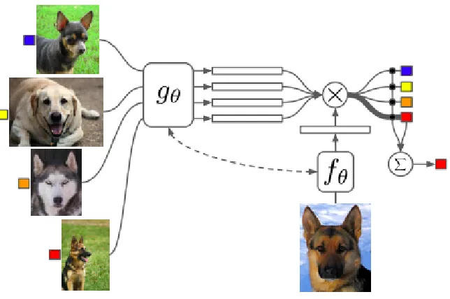
Jake Snell et al. [29] proposed the Prototypical Networks, which is based on the idea that

each class can be represented by the mean of its supporting examples in a representation space

learned by a neural network. When one query comes, its classification can be performed by

computing distances to prototype representations of each class. Figure 2.8 shows the

Prototyp-ical networks in the few-shot and zero-shot scenarios.

Flood Sung et al. [31] proposed the Relation Network, which is designed to learn a deep

distance metric to conduct few-shot learning within episodes. In each episode, the network

is designed to simulate the few-shot setting. After training, the relation network is able to

classify images of new classes by computing relation scores between query images and the few

supporting examples of each new class. Figure 2.9 shows the relation network architecture for

a 5-way 1-shot problem with one query example.

The most related methods to ours are the Relation Networks [31] and the Convolutional

Siamese Networks [18]. These approaches focus on learning embeddings in which images are

represented, such that it can be easily recognized using a fixed nearest-neighbor [29] or linear

(30)

2.3. Regions ofInterestSelection 19

Network, replacing the fixed metric on the top of the Convolutional Siamese Network for the

relation classifier CNN in Relation Network. Therefore, our method can provide a learnable

rather than fixed metric, or non-linear rather than linear classifier.

2.3 Regions of Interest Selection

Regions of Interest selection is also called object proposal in some papers. It has been widely

used in the object detection area. Comprehensive surveys and comparisons about RoIs

selec-tion methods can be found in these papers [13, 5]. To sum up, Regions of Interest selection

methods could be divided into two approaches: one method is based on grouping superpixels

(e.g., selective search [33]). Another method is based on sliding windows (e.g., objectness

in windows [1], EdgeBoxes [35]). Many object proposal methods, like selective search, have

been used as an independent detector module. In this paper, we use selective search method to

obtain the Regions of Interest because selective search that is used as an independent detector

(31)

Chapter 3 Methodology

In this chapter, we explain our approach for few-shot learning same-different visual problems

in detail. Firstly, we analyze the problem that we need to solve and define it as one-shot

learning in a broad sense, and then we describe our model and each module in the model in

detail. Lastly, we briefly introduce how our model learns on training samples.

3.1 Problem Definition

We try to solve the same-different problems with few-shot learning. According to the previous

research on few-shot learning, we need to use three datasets: a training set, a supporting set,

and a testing set. The support set and testing set share the same label space. They are from

the target few-shot problems. With the support set only, we can, in principle, train a classifier

to predict a class labelyfor each sample xin the test set. However, due to the lack of labeled

samples in the support set, it will cause over-fitting, and the performance of such a classifier

is usually not satisfactory. Therefore, we need to use the training set to perform the

meta-training tasks in advance. The meta-training set has its own label space that is different from the

support and testing set, and is mainly used to perform the meta-training such that transferable

knowledge can be learned to help to perform better few-shot learning on the support set and

classify the test set more effectively. When the support set contains C distinct classes and

(32)

3.2. Model 21

K examples in each class, the target few-shot problem is called C-wayK-shot. Considering

SVRT SD problems consisting of randomly generated objects in each class of each task (e.g.

for SVRT #1, although Class 2 contains two same objects in each image, the same objects are

different among the images, as shown in Figure 3.1), we need to learn the similarity between

the objects for each image when solving this problem. Therefore, we can define the problem

we are studying as one-shot learning, which means that the machine needs to predict whether

another object is the same as this object that machine only saw once.

Figure 3.1: A few samples in “sameness” class for SVRT #1

3.2 Model

In order to solve the SVRT SD problems, we built a novel model. Our model consists of three

parts: 1) Regions of Interest selection module. 2) same-different twins network. 3) pattern

recognition module. Figure 3.2 illustrates the simplified process in solving the SVRT

same-different problems through our approach. Firstly, samples xi are entered into the regions of

interest selection module, resulting in a set of regions of interest (ri, rj,...). Then randomly

grouping these regions of interest into pairs and feeding each pair into the same-different twins

network. Same-different twins network is developed based on the Convolutional Siamese

Neu-ral Network [18] through replacing the fixed L1 distance metric on the top of the siamese

network to a learnable CNN metric. Same-different twins network contains two modules: an

(33)

22 Chapter3. Methodology

embedding module fϕ, which produces feature maps fϕ(ri) and fϕ(rj). The feature maps fϕ(ri)

and fϕ(rj) are combined with operatorC(fϕ(ri), fϕ(rj)). In this work, we assume C(., .) to be

the concatenation of feature maps in depth. The combined feature map of the pair is fed into

the relation modulegφ, which eventually produces a scalar in range of 0 to 1 representing the

similarity for each pair such as ri and rj, which is called relation score. The relation score

betweenri andrj is gφ(C(fϕ(ri), fϕ(rj))). After that, we use the pattern recognition module to

determine which class samplesxibelongs to based on these relation scores. The pattern

recog-nition module includes a filter module p and a k-nearest classifier. The filter module p sets

the relation scores below the threshold to 0 and then adds all theses relation scores to obtain a

similarity value. Finally, we use a k-nearest neighbor classifier to predict the class label based

on the similarity value for each test image.

Figure 3.2: The simplified process in solving the SVRT SD problems through our approach

3.2.1 Regions of Interest Selection Module

To locate the objects in the image, we use the selective search method [33] to obtain

(34)

3.2. Model 23

Python-OpenCV. Selective search combines the advantages of both an exhaustive search and

segmentation, and it can capture all possible object locations with high recall. Selective search

has been developed as an independent detector. There are three hyper-parameters in the

se-lective search method: scale, sigma and minSize. Objects can be effectively located through

configuring reasonable parameters for the hyper-parameters sigma, scale, minSize. In all

de-tection results, some dede-tection results are inaccurate and highly repetitive. In order to remove

duplicate regions and improve detection accuracy, we calculate the Intersection-over-Union

(IoU) among regions. In mathematics, IoU is a statistic used for gauging the similarity and

diversity of sample sets. In the field of the image, IoU is a standard for measuring the detection

accuracy of a corresponding object. The method of calculating IoU in the field of the image is

showed in Figure 3.3. It means that the area where the two detection regions overlap is divided

by the total area. We set a threshold to remove the inaccurate detection results for SVRT SD

problems. When the IoU between two regions is greater than the threshold, the region with the

smaller area is removed. Each bounding box is defined by a four-tuple (r,c,h,w) that specifies

its top-left corner (r,c) and its heighthand widthw.

(35)

3.2.2 Same-di

ff

erent Twins Network

Same-different twins network is developed based on the Convolutional Siamese Neural

net-work [18]. As we have known, metric-learning based approaches aim to learn a set of

projec-tion funcprojec-tions such that when images are represented in the embedding space, they are easy to

recognize using simple nearest neighbor or linear classifiers [34,29,18]. In the Convolutional

Siamese Neural network [18], the authors used theL1 distance metric to compute the distance

between the highest level feature representations of each pair. In this work, we use a

learn-able CNN metric called relation module to replace the L1 distance metric. Compared withL1

distance that focuses on learning a shallow (linear) Mahalanobis metric for fixed feature

rep-resentation, the CNN metric can learn a deep non-linear metric (similarity function) that can

better identify matching/mismatching pairs. This has been shown in [31]. We also developed

a new embedding module that can accommodate the 84 x 84 SVRT images.

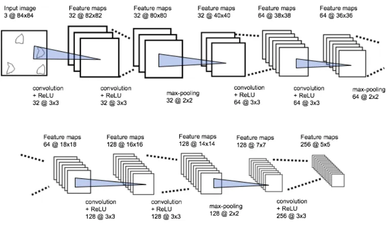
Figure 3.4 shows the convolutional architecture for the embedding module. VGG16 is a

convolutional neural network model proposed by K. Simonyan and A. Zisserman from the

University of Oxford in [28]. The model achieves 92.7% top-5 test accuracy in ImageNet,

which is a dataset of over 14 million images belonging to 1000 classes. We developed a

VGG-like architecture for the embedding module. The embedding module consists of a sequence

of convolutional layers and max-pooling layers. The convolutional layers have filters of size

three and a fixed stride of 1. The number of convolutional filters is specified as a multiple of

16, which refers to the Convolutional Siamese Neural network [18]. This setting can optimize

the performance of extracting features. The embedding applies a rectified linear units (ReLU)

activation function to the outputted feature maps. Each set of convolutional layers is followed

by a 2x2 max-pooling layer with the stride of 2.

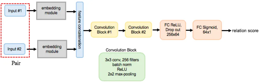
After obtaining the feature maps of the twin pairs through the embedding module, the

fea-ture maps are concatenated in-depth and inputted into the relation module. Figure 3.5 shows the

relation module for few-shot learning same-different problems. The relation module consists

(36)

con-3.2. Model 25

Figure 3.4: Convolutional architecture for the embedding module

tains a convolution layer with 256 filters followed by batch normalization, ReLU non-linearity

activation function, and a 2x2 max-pooling layer. Each filter in the convolution layer has the

kernel size of 3x3. Two convolutional blocks are followed by two fully-connected layers. The

two fully-connected layers are 64 and 1 dimensional, respectively. The first fully-connected

layer uses the ReLU activation function, and the output layer uses the Sigmoid activation

func-tion (logistic funcfunc-tion) in order to generate relafunc-tion scores in a reasonable range for each twin

pair. Between the two fully connected layers, we added a dropout layer that helps alleviate

over-fitting.

3.2.3 Pattern Recognition Module

Some SVRT tasks contain more than two objects and need to solve the highly abstract concept

of “grouping” such as SVRT #5 and SVRT #7. For SVRT #7, objects in the positive class can

be organized into three groups, each containing two same objects. Objects in the negative class

(37)

Figure 3.5: Relation module for few-shot learning SD problems

to identifying the sameness and difference for each pair, we also need to learn the pattern in

each class. As discussed, through a same-different twins network, we can obtain the relation

score for each pair and finally get all relation scores for all pairs. Based on the relation scores, a

simple method to recognize the pattern for each class is to get the sum of these relation scores.

However, due to that SVRT images are too simple, just composed of lines, many pairs that

belong to different classes also have very high relation scores. Therefore, we need to use a

threshold, which is obtained through training set and validation set, to distinguish the relation

scores. When relation score is below the threshold, this pair has a high probability of belonging

to a different class, and we set the relation score of this pair to 0. After that, we obtain the sum

of all the relation score as the similarity value. In this way, we can use simple nearest neighbor

or linear classifiers to recognize the class due to that the similarity is one-dimensional and can

reflect the pattern for each class. Finally, we train a k-nearest neighbor classifier to predict

class labels based on the similarities.

3.3 Learning

Loss function. Letiindexes theith mini-batch (the number of training data during one

itera-tion). Suppose the min-batch size ism. Lety(xi

1,x

i

(38)

3.3. Learning 27

vector refers to the true label of the mini-batch. When x1 andx2 belong to the same category,

y(xi₁,xi₂) = 1, otherwisey(xi₁,xi₂) = 0. Let vector p(xi₁,xi₂) withm length represents the

pre-dicted results for the mini-batch. We used the binary cross-entropy as the loss function. Binary

cross-entropy can be calculated as:

L(xi₁,xi₂) = −y(xi₁,xi₂)logp(xi₁,xi₂)−(1−y(xi₁,xi₂))log(1− p(xi₁,xi₂)) (3.1)

Optimization. Backpropagation is an algorithm widely used in the training of feedforward

neural networks for supervised learning. In this work, we also use the standard

backpropaga-tion algorithm to optimize our object funcbackpropaga-tion by calculating the gradient. We set the

mini-batch size to 128 with learning rateαj, momentumβjand regulation weightsλj, so the update

rule at epochT is as follows:

wkTj(x i

1,x

i

2) = wkTj + ∆wkTj(x i

1,x

i

2)+2λj|wk j| (3.2)

∆wkTj(x i

1,x

i

2) = −αj5wkTj +βj∆wkTj−1 (3.3)

where5wk j is partial derivative with respect to the weight between the jth neuron in some

layer and thekth neuron in the successive layer.

Weight initialization. Before the training, we initialized the weights and biases for all

convolution layers and fully-connected layers. For all convolution layers, the weights were

drawn from a normal distribution with zero mean and a standard deviation of 10−2_{. The biases}

were initialized from a normal distribution with the mean 0.5 and a standard deviation of 10−2_.

The fully-connected layers were initialized in the same way as the convolution layer, but the

weights were initialized using a normal distribution with zero mean and a standard deviation

of 2x10−1_.

Learning rate. In this work, we set the initial learning rate to α, and the learning rate is

gradually decreased following the method of dividing by 10. For example, assume that the

(39)

monitored the one-shot validation error when training the same-different twins network. When

the validation accuracy did not increase for 50 iterations, we stopped and used the parameters

of the model at the best iteration step according to the one-shot validation accuracy. Then we

updated the learning rate to continue to train the network.

Hyperparameter optimization. For the learning rate and regularization

hyperparame-ters, we set the initial learning rateα[10−2,10−1], momentumβ[0,1], and regulation weights

λ[0,0.1]. For neural network hyperparameters, we set the number of convolution filters in

each layer from 16 to 256 using multiples of 16. For the fully connected layer

hyperparam-eters, we set the units from 16 to 256, also in multiples of 16. These hyperparameters are

(40)

Chapter 4 Experiments

In this chapter, we first discuss the experimental setup, including the datasets that we used and

the performance evaluation method, several strong baselines, and some experiment

implemen-tation details. Then, we present the experimental results of our approach and compare them

against the strong baselines. After that, we analyze the experimental results in detail.

4.1 Datasets

We use the meta-learning (learn to learn) strategy to solve the same-different problems with

few-shot learning. According to the previous research on meta-learning, we need to use two

kinds of datasets. The first data set is used for meta-training to extract some transferable

knowledge from some auxiliary tasks such that it can help the model to learn the generalization

ability. The second data set is the dataset for meta-testing, which is the SVRT problems that

we currently need to solve.

4.1.1 Meta-training datasets

In this thesis, we use the Omniglot dataset as the meta-training dataset to extract some

transfer-able knowledge. Omniglot dataset was collected by Brenden Lake and his collaborators [20]

(41)

30 Chapter4. Experiments

Figure 4.1: The Omniglot dataset contains different images from alphabets across the world.

and was used for studying one-shot learning and for developing more human-like learning

al-gorithms. Omniglot contains over 1600 handwritten characters from 50 different alphabets

ranging from familiar Latin to unfamiliar local dialects. Figure 4.1 shows a few examples from

the Omniglot dataset. Omniglot dataset can be obtained from the github1_{or downloaded from}

www.omniglot.com.

The number of characters (classes) in each alphabet varies considerably from about 15 to

upwards of 40 characters. Each class contains 20 samples drawn by different people. Lake split

the 50 different alphabets into a 40 alphabet background set and a 10 alphabet evaluation set.

The background set is used for developing the same-different twins network by learning

hyper-parameters and feature mappings. The evaluation set is used to test the one-shot classification

performance of the network. Each image in Omniglot dataset is a 105x105 binary-valued image

which was drawn by hand on an online canvas. In order to transfer the developed twins network

to solve the SVRT problems, we resize the Omniglot dataset to 84x84 to keep consistent with

SVRT tasks. We also change the binary-valued image to the RGB image due to images in

SVRT tasks have an RGB image format.

Besides, considering that each class only contains 20 samples, we also augmented the

(42)

4.1. Datasets 31

Figure 4.2: A few samples of random data augmentation generated for three images in the Omniglot data set

ground set (training set) with the data augmentation, which is a strategy that can significantly

increase the diversity of data available for training models, without actually collecting new

data. The data augmentation techniques include scaling, rotation, horizontal flipping, and

translation. Figure 4.2 shows a few samples of random data augmentation generated for three

images in the Omniglot data set.

4.1.2 SVRT datasets (meta-testing datasets)

In this thesis, we try to solve the SVRT same-different visual reasoning problems. This series

of synthetic image recognition problems is developed by Fleuret and Don Geman. The code

to generate these SVRT tasks is publicly available at2. Figure 1.2 in Chapter 1 shows a few

examples of the SVRT SD problems. For each task, we use ten labeled training samples, 1000

validation sets, and 10000 test samples in order to compare our method with the published

results by Fleuret et al. [10] where the authors used ten training samples. We also augmented

the training sets with small affine distortions. The affine distortions include scaling and rotation.

The augmented training sets are mainly for training the pattern recognition module.

2

(43)

4.2 Performance Evaluation Method

There are various metrics that can be used to evaluate machine learning algorithms. These

metrics include classification accuracy, F1 Score, confusion matrix, and so on. In this thesis,

we use the classification accuracy to evaluate the performance of our model. Classification

accuracy is the ratio of the number of correct predictions to the total number of input samples.

For every SVRT SD task, we conducted ten testing trials and used 1000 test samples for each

test trial (including 500 positive samples and 500 negative samples). The final performance is

the mean of classification accuracy for ten testing trials.

4.3 Implementation Details for Our Method

We solved the SVRT SD problems in three steps. The first step is to select the Regions of

Interest by the selective search. The second step is to meta-training the same-different twins

network. The last step is to use the trained same-different twins network to do one-shot learning

and predict the relation score for each pair of regions of interest. After that, the pattern

recog-nition module is used to do the classification task for SVRT same-different problems based on

the predicted relation scores.

For the selection of Regions of Interest, we set the hyper-parameters scale to 1000, sigma

to 0.3, and min size to 10, which helps to locate the objects effectively. For the IoU, we set

the threshold to 0.9, which means that when the IoU between two regions of Interest is greater

than 0.9, the region with the smaller area is removed.

For the same-different twins network, we used the Omniglot dataset for meta-training,

which helped the same-different twins network learn some transferable knowledge. Firstly,

randomly grouping the Omniglot background set into pairs, and then these pairs were fed into

the same-different twins network to train this network. Hyper-parameters follow the setting

below: batch size 128, Adam optimizer (the initial learning rate 0.06, momentum 0.6,

(44)

4.4. Baselines 33

network [18], and we set 1000 validation tasks for each evaluation to help us select the optimal

parameters. The network with the maximum classification accuracy was used to predict the

similarity of Regions of Interest on SVRT SD tasks. The same-different twins network was

implemented with PyTorch.

Finally, the pattern recognition module was used to predict the class for new SVRT SD

samples based on the similarities of Regions of Interest. Firstly, the pattern recognition module

filtered the relation scores and set the relation scores below the threshold to 0. The threshold

was learned through the SVRT SD validation set, selecting the value which had maximum

classification accuracy on the validation set. After that, the similarity value for each image was

obtained by adding the relation scores of all these pairs of regions of interest. Then we trained

a k-nearest neighbors classifier to predict class labels for each new SVRT image based on the

similarities. The value fork was chosen from{1,2,3,4,5}and the best value was found to be

k= 2.

4.4 Baselines

Apart from comparing to the few-shot learning results for SVRT same-different tasks obtained

by Fleuret et al. [10], we also compare our method against several other approaches known

to perform well at other few-shot classification tasks, including fine-tune deep CNNs,

Model-Agnostic Meta-Learning (MAML) [9], Prototypical Nets [29], and Relation Nets [31]. For

all these models, we used SVRT images of size 84x84, ten training samples,1000 validation

samples, and 10000 test samples. Performance is measured with classification accuracy. To

produce all experimental results, we average across ten trials, with 1000 different unseen test

images each trial. For hyper-parameter tuning, we used 1000 validation images for every task.

In addition, for meta-learning methods Model-Agnostic Meta-Learning (MAML) [9],

Pro-totypical Nets [29], and Relation Nets [31], we also used Omniglot datasets to do the

(45)

SD tasks in the meta-testing phase. Due to that each SVRT task is a binary classification

ques-tion and has 10 training samples (5 positive, 5 negative), we defined the meta-learning tasks as

2-way 5-shot. The 2-way 5-shot meta-training tasks were generated through Omniglot datasets.

2-way 5-shot meta-testing tasks were also generated by SVRT SD problems(10 training

sam-ples, 10000 testing samples).

4.4.1 Fine-tune deep CNNs

Fine-tune deep CNNs is mainly the reuse of a pre-trained model on a new problem. When

solving a new problem, most of the layers in front of the model are frozen, and we only need to

fine-tune the last few layers. For this method, we fine-tuned the Vgg-16 architecture pre-trained

on ImageNet [28]. Other architectures are also possible such as ResNet, InceptionV3,

Xcep-tion. The fully connected layers in Vgg-16 architecture were replaced by two fully-connected

layers with width 256 and 64 activated by sigmoid function. The softmax classifier was trained

with the Adam optimizer provided by Keras, and the loss function used binary cross-entropy

loss. We trained the deep CNNs for 200 epochs, and the optimal number of epochs for each

SVRT same-different task was chosen based on the classification accuracy on validation set.

The optimal number of epochs for each task was chosen from{8,16,32,64}.

4.4.2 Model-Agnostic Meta-Learning

MAML aims to meta-learn an initial set of neural network weights (the parameters of the

model are explicitly trained), so the neural network models can be effectively fine-tuned to

pro-duce good generalization performance on the new few-shot learning tasks within few

gradient-descent update step. We used the same architecture for this approach, as in Finn’s article. The

implement process is publicly available in 3_{. 2-way 5-shot meta-training tasks are generated}

through Omniglot datasets. We set 60000 meta-train iterations and used 1000 validation

im-ages for each task. Finally, we selected the model that maximized the prediction accuracy on

(46)

4.4. Baselines 35

SVRT SD validation images to test the 10000 different unseen SVRT SD images for each task

for ten trials (1000 test samples for one trial).

4.4.3 Prototypical Network

Prototypical network is developed based on the idea that each class can be represented by the

mean of its supporting examples in a representation space learned by a neural network on the

meta-training tasks. We used the same architecture for this approach, as in Snell’s article [29].

The implement process is publicly available in4. Omniglot datasets were used to do the 2-way

5-shot meta-learning task for the Prototypical network. Ten training samples in SVRT tasks

were used as the supporting set. Finally, we predict the class for the 10000 SVRT SD test

samples for ten trials (1000 test samples for one trial). The optimal number of epochs for each

task was chosen from{8,16,32,64}.

4.4.4 Relation Network

Relation network is designed to learn a deep distance metric through simulating the few-shot

setting in each episode. For this model, we used the same CNN architecture and Relation

Network architecture in Sung’s article [31]. The implement process is publicly available in5_.

Omniglot datasets were used to do the 2-way 5-shot meta-learning task for the Relation

Net-work. Ten training samples in SVRT tasks were used as the supporting set. Finally, the class

was predicted for the 10000 test samples in SVRT SD tasks for ten trials (1000 test samples for

one trial) by using the trained model. The batch number for each class is set to 5. The training

episode and test episode are separately 10000 and 1000.

4_{https://github.com/jakesnell/prototypical-networks}

(47)

Figure 4.3: Examples of the fifth-layer convolutional filters learned by same-different twins network.

4.5 Experiment results

Our experimental results include two parts: one is for meta-training on Omniglot dataset, and

another part is for meta-testing on SVRT same-different problems.

4.5.1 Experiment Results for Meta-training

As mentioned before, we used the meta-learning strategy to train the same-different twins

network. Table 4.1 shows the meta-training experiment results for the same-different twins

network on Omniglot dataset. Due to that our same-different twins network was developed

based on the Siamese network [18], we also compared the 20-way one-shot performance of

our network to the Siamese network, as showed in Table 4.1. It can be observed that our

same-different twins network greatly improves the one-shot classification accuracy for nearly 5%,

compared with the Siamese network.

Method Test

Siamese network 92.0

Same-different twins network 96.7

Table 4.1: Comparing the one-shot accuracy between the Siamese network and Same-different twins network.

(48)

4.6. ExperimentResultsAnalysis 37

can be noticed that different filters have different effects. Some filters may look for very small

point-wise features, while some filters may act as the larger scale edge detectors.

4.5.2 Experiment Results for SVRT SD Problems

Table 4.2 contains the performance for each method on the SVRT same-different problems.

All results are averaged across ten trials except the results from Fleuret et al. [10], where the

number of trials is unknown. All results, except GoogLeNet and Human performance, were

obtained with only ten training samples. GoogLeNet used 20000 training examples. The

human performance showed in Table 4.2 was estimated by Stabinger et al. [30] based on the

original data reported by Fleuret et al. [10]. The average numbers of images required to learn

the rules for humans for each SVRT SD task were reported by Fleuret et al. [10] and shown in

the Figure 2.2 in Chapter 2.

The meanings of model acronyms in table 4.2 are as follows: Fleuret: The Adaboost and

spectral features model from Fleuret et al. [10]. PN: Prototypical Network. RN: Relation

Network. Vgg-16: Fine-tune deep CNNs, pre-trained Vgg-16 for feature extraction. MAML:

Model-Agnostic Meta-Learning. GoogLeNet: Performance of GoogLeNet on the SVRT SD

problems, published results from the paper [30]. Human: Estimated accuracy of participants,

and human tests were done by Fleuret et al. [10].

4.6 Experiment Results Analysis

The most immediate observation from Table 4.2 is the performance difference between our

approach and all other models we compare against. It can be observed that our model greatly

outperforms other models on all SVRT same-different problems with an average advantage

of above 35% when only provided with ten training samples. On some SD problems such

as SVRT #5, #15, and #16, our method even surpasses the reported performance of human

A New Method to Solve Same-different Problems with Few-shot Learning

Scholarship@Western

Scholarship@Western

A New Method to Solve Same-different Problems with Few-shot

A New Method to Solve Same-different Problems with Few-shot

Learning

Learning

Abstract

Summary for Lay Audience

Acknowlegements

Contents

List of Figures

List of Tables

Chapter 1

Introduction

1.1

Background

1.2

Research Question

1.2.1

SVRT Visual Reasoning Tasks

1.2.2

Other Same-di

ff

erent Problems

1.3

Contributions

1.4

Structure of this Thesis

Chapter 2

Related Work

2.1

Research on Same-di

ff

erent Problems

2.1.1

Same-di

ff

erent Visual Reasoning Tasks

2.1.2

Standard Same-di

ff

erent Classification Tasks

2.2

Few-shot Learning Methods

2.2.1

Few-shot Learning based on Fine-Tuning

2.2.2

Few-shot Learning based on RNN Memory

2.2.3

Few-shot Learning based on Embedding and Metric Learning

2.3

Regions of Interest Selection

Chapter 3

Methodology

3.1

Problem Definition

3.2

Model

3.2.1

Regions of Interest Selection Module

3.2.2

Same-di

ff

erent Twins Network

3.2.3

Pattern Recognition Module

3.3

Learning

Chapter 4

Experiments

4.1

Datasets

4.1.1

Meta-training datasets

4.1.2

SVRT datasets (meta-testing datasets)

4.2

Performance Evaluation Method

4.3