Scholarship@Western
Scholarship@Western
Electronic Thesis and Dissertation Repository
6-20-2019 2:00 PM
A computationally efficient methodology in pricing a guaranteed
A computationally efficient methodology in pricing a guaranteed
minimum accumulation benefit
minimum accumulation benefit
Yiming Huang
The University of Western Ontario
Supervisor
Mamon, Rogemar
The University of Western Ontario
Graduate Program in Statistics and Actuarial Sciences
A thesis submitted in partial fulfillment of the requirements for the degree in Master of Science © Yiming Huang 2019
Follow this and additional works at: https://ir.lib.uwo.ca/etd
Part of the Statistics and Probability Commons
Recommended Citation Recommended Citation
Huang, Yiming, "A computationally efficient methodology in pricing a guaranteed minimum accumulation benefit" (2019). Electronic Thesis and Dissertation Repository. 6507.
https://ir.lib.uwo.ca/etd/6507
This Dissertation/Thesis is brought to you for free and open access by Scholarship@Western. It has been accepted for inclusion in Electronic Thesis and Dissertation Repository by an authorized administrator of
In this thesis, we consider a framework under which three correlated factors, namely, finan-cial, mortality and lapse risks, are modelled in an integrated way. This modelling framework supports the valuation of a guaranteed minimum accumulation benefit (GMAB). The change-of-measure approach is employed to come up with a compact and implementable valuation expressions. We provide a numerical demonstration to confirm the efficiency and accuracy of our proposed pricing methodology. In particular, our approach on average takes only 0.07% of the computing time entailed by the Monte-Carlo (MC) simulation technique. Furthermore, the standard errors of our approach’s results are lower than those obtained from MC-based com-putations. When there are no renewal options in a GMAB contract, we get the special case of a guaranteed minimum maturity benefit for which a closed-form pricing solution is derived.
Keywords: Variable annuities, investment guarantee, stochastic model, change of proba-bility measures
When a customer comes to an insurance company to learn something about one specific in-surance product, the insurer will be asked to provide the corresponding purchase price. After obtaining the customer’s essential information, they start to calculate the price. However, if they can’t give a response within a short time, they would provide a negative customer ser-vice experience, which consequently might force the customer to switch to another company. Therefore, it is important for the insurer to have a quick-response evaluation system in order to get an edge over the competition. This thesis will provide such an evaluation framework in the valuation of a specific insurance product, called the guaranteed minimum accumulation benefit (GMAB).
I would like to convey my profound gratitude to my supervisor, Dr. Rogemar Mamon, for his enthusiasm, scientific guidance, and for sharing his expertise and experiences throughout my research training at Western. His careful editing and research insights contributed enor-mously to the production of this thesis.
I would like to express my sincere thanks to my thesis examiners, Dr. Hao Yu, Dr. Marcos Escobar-Anel and Dr. Simon Bonner, for taking the time out of their their busy schedule to read my thesis. Their constructive and useful comments are very much appreciated.
I take pleasure in thanking my colleagues and friends, Dr. Yixing Zhao and doctoral can-didates Xing Gu, Yifan Li and Junhe Chen, for their valuable assistance and ideas.
Last but not least, my heartfelt appreciation goes to my family, for their love and constant support. This thesis would not have been possible without their encouragement.
Abstract ii
Lay Summary iii
Acknowledgements iv
List of Figures vii
List of Tables viii
1 Introduction 1
2 Modelling framework 3
2.1 Interest rate model. . . 3
2.2 Mortality model . . . 4
2.3 Lapse rate model . . . 4
2.4 Model dependence . . . 5
3 Contract description 6 3.1 Guaranteed Minimum Accumulation Benefit . . . 6
3.2 Guaranteed Minimum Maturity Benefit. . . 7
4 Derivation of valuation formula 9 4.1 The forward measure . . . 9
4.2 The survival measure . . . 10
4.3 The endowment-risk-adjusted measure . . . 11
4.4 Valuation formula . . . 12
5 Numerical illustration 20
5.1 Numerical scheme. . . 20
5.2 Price-sensitivity analyses . . . 24
6 Conclusion 28 Bibliography 30 Appendices 33 Appendix A Calculation details for the dynamics ofΛ3(k) t underQ 34 Appendix B Calculation details for the covariances in Chapter 4 37 Appendix C Codes for GMAB evaluation 40 C.1 Codes for the direct approach in the GMAB evaluation . . . 40
C.2 Codes for our proposed method in the evaluation of GMAB . . . 44
Appendix D Codes for GMMB evaluation 51 D.1 Codes for the computation of GMMB value using the direct approach . . . 51
D.2 Codes for the computation of the GMMB under our proposed method . . . 54
Appendix E Codes in conducting price-sensitivity analyses 59 E.1 Codes for Figure 5.1 . . . 59
E.2 Codes for Figure 5.2 . . . 61
E.3 Codes for Figure 5.3 . . . 62
E.4 Codes for Figure 5.4 . . . 63
Curriculum Vitae 65
5.1 GMAB prices under different parameter values . . . 25
5.2 GMAB prices under different parameter values . . . 26
5.3 GMMB prices with various values of maturityT3 . . . 26
5.4 GMAB prices versus varyingT1andT2 . . . 27
5.1 Parameter values . . . 22 5.2 GMAB prices calculated using equations (3.3) and (4.28) . . . 23 5.3 GMMB prices calculated utilising equations (3.4) and (4.16) . . . 24
Introduction
With a population expected to live much longer into the future, the popularity of a variable annuity has grown rapidly over the years. According to the First-Quarter 2019 U.S. Retail An-nuity Sales Survey conducted by the LIMRA Secure Retirement Institute (LIMRA SRI) [12], variable annuity (VA) sales from January-March 2019 totaled $22.8 billion. These represent 37.5% of overall annuity sales; it is the highest figure for a first-quarter total annuity sales going back for a decade.
A variable annuity is a tax-deferred contract between a policyholder and an insurance com-pany. The benefits to the policyholder will depend on the performance of the investment funds provided by the insurance company; typically, the benefit is the greater of the account value and the guaranteed amount. Contracts typically contain certain guarantee riders offered by the in-surance company in order to afford different types of financial protection. There are two major types of guarantee riders: guaranteed minimum death benefits (GMDB) and guaranteed min-imum living benefits (GMLB). The GMLB consists of three main subcategories: guaranteed minimum accumulation benefits (GMAB), guaranteed minimum income benefits (GMIB), and guaranteed mnimum withdrawl benefits (GMWB). A detailed overview of a variable annuity is given in Gan [6].
Even though GMAB is a simple living benefit, it differs from the other living benefit riders in terms of the risk posed to the insurance company. It is crucial for an insurance company to scrutinise the contracts with a GMAB rider. This is because there is a need to follow up the detailed fund performance information, reset the guarantee amounts, and pay the difference
amounts to the segregated fund at renewal dates.
Bauer et al. [2] provided a comprehensive mathematical model for modelling and valua-tion of many types of variable annuity riders. A unifying framework is proposed in Bacinello et al. [1] for valuing variable annuity guarantees using a Monte-Carlo (MC) method. In Doyle and Groendyke [5], the use of neural networks is explored to price variable annuity guaran-tees. Nonetheless, many papers dealing with this problem do not take into consideration the correlation between interest and mortality rates, and they do not consider lapsation as a risk factor as well. Although this paper employs the modelling framework in Zhao and Mamon [21], which synthesises interest, mortality and lapse rates altogether for a guaranteed annuity option pricing, the efficient valuation of GMAB has its own peculiarity and challenges, which requires a separate and focused analysis being addressed by this methodological and empirical study.
Modelling framework
We assume that our valuation framework is supported by a filtered probability space (Ω,F,{Ft},Q). Here,{Ft}is the joint filtration generated by the interest ratert, force of mortalityµt and lapse ratelt, andQis a risk-neutral probability measure.
2.1
Interest rate model
As specified above, it is supposed thatQexists and the dynamics ofrt is given by the Vasiˇcek model
drt =a(b−rt)dt+σ1dXt, (2.1)
wherea,bandσ1are positive constants, andXt is a standard Brownian motion (BM) underQ. Such aQis equivalent to an objective measureP, under which the realisations or some proxies for the realisations of our underlying variables are observed.
Apparently, this model can generate negative interest rate values; nonetheless this feature accommodates the occurrence of negative rates in situation when monetary authorities have to combat deflation by encouraging people and businesses to spend money rather than keep it safe in the banks. For instance, the European Central Bank introduced a negative interest-rate policy in 2014 whilst the Bank of Japan did the same in 2016 to stimulate its economy and overcome persistent deflationary pressures in its economy. The price B(t,T) of aT-maturity
zero-coupon bond at timet <T (cf Mamon [18]) is given by
B(t,T)= EQ
e−
RT
t rudu
Ft
= e−A(t,T)rt+D(t,T), (2.2)
where
A(t,T)= 1−e
−a(T−t)
a
and
D(t,T)= b− σ
2 1
2a2
!
[A(t,T)−(T −t)]− σ
2 1A(t,T)
2
4a .
2.2
Mortality model
The force of mortalityµx,tat timetfor an individual agedxat time 0 is governed by a non-mean reverting OU process, as proposed to Luciano and Vigna [17], and it has dynamics
dµt = cµtdt+ξdYt, (2.3)
wherecandξare positive constants, andYt is a standard BM. Noting that our emphasis is the dynamics with respect to the passage of time, we shall simply use µt to representµx,t in the succeeding discussion to avoid clutter of notation. Then, we recall the survival function
S(t,T)=EQ
e−
RT
t µudu
Ft
.
2.3
Lapse rate model
Lapse risk is the possibility that policyholders terminate their policies that arises from surren-dering or stopping to pay premiums, which could cause huge losses and liquidity problem to the insurers. Therefore, it is another essential factor in pricing insurance products. Letlt be the lapse rate at timet,and assume that it evolves as a mean-reverting process similar to the setting in Zhao and Mamon [21]. That is,
dlt = h(m+prt−lt)dt+ζdZt, (2.4)
2.4
Model dependence
The works by Liu et al. [15] argued that the correlation between interest rate and mortality rate has significant effect in pricing annuity products, thus it must be incorporated in our valuation framework. In particular, as noted in the findings of Dhaene et al. [4], dependence modelling in a risk-neutral pricing world is necessary to give allowance to correlated financial and acturial risks despite their being independent in the real world. Secondly, Kuo et al. [14] used the co-integration technique in the investigation of the contending-lapse-rate hypotheses that tackles the tension between the emergency fund hypothesis and the interest rate hypothesis. It was found that the interest rate has a statistically significant power in explaining the long-term behaviour of the lapse rate as over the long run, it causes lapse rate’s variations. Hence, the correlation between interest rate and lapse rate must be considered. Thirdly, a contract policy’s lapsation could be linked to mortality or morbidity-adverse selection. This means that policy holders who are in adverse health or have other insurability problems tend not to lapse their policies; this is because they will have difficulty finding comparable insurance coverage at the same premium level. Thus, we need to take into consideration the interaction between mortality rate and lapse rate. Simply put, decisions on whether to continue life insurance policies are influenced by the insureds’ perceived likelihood of survival.
We assume thatXt,YtandZtare correlated and their dependence is modelled as
dXtdYt = ρ12dt, dXtdZt =ρ13dt and dYtdZt =ρ23dt.
Their explicit specifications are as follows:
dXt = dWt1, dYt = ρ12dWt1+
q
1−ρ2 12dW
2
t,
dZt = ρ13dWt1+ρ
0
23dW 2
t +
q
1−ρ213−ρ0232dWt3,
whereWt1,Wt2 andWt3 are independent standard BMs and
ρ0
23=
ρ23−ρ12ρ13
q
1−ρ2 12
. (2.5)
Contract description
In this chapter, we present the detailed contract description of a GMAB.
3.1
Guaranteed Minimum Accumulation Benefit
Denote byM(t,T) the fair value at timetof a $1 pure endowment payable at maturityT under a two-decrement model (both mortality and lapse rates are considered). From the risk-neutral pricing principle,
M(t,T)=EQ
e−
RT
t rudue−
RT
t µudue−
RT
t ludu
Ft
. (3.1)
The value of M(t,T) is needed in our succeeding analysis of a GMAB, which is a contract that guarantees the policyholder a specific monetary amount at maturity, provided that the policyholder is still alive at the contract’s maturity. Moreover, the policyholder has the option to renew the contract at some renewal dates, at a new guarantee level. Further descriptions on the design of a GMAB can be found in [9].
In this thesis, we assume two renewals atT1andT2, and the maturity atT3(clearly this can
be adapted to more renewals). The guaranteed valueGt is assumed to have a roll-up feature, i.e.,
Gt = P0eδt,
whereP0 is the contract’s initial single premium, andδ is a predetermined roll-up rate; when
δ =0 we are in the situation called return of premium. The segregated fundFt is linked to the
performance of a stock indexSt and this is expressed as
Ft = F0
St
S0
e−αt,
whereαis the constant continuously compounded management charge rate, andF0= S0 = P0.
The stock indexSt follows a geometric BM; so
dSt = rtStdt+σ2StdWt4,
where σ2 is a positive constant, and Wt4 is a standard BM independent of Wt1, Wt2 and Wt3. Applying Itˆo’s lemma, it can be shown that the dynamics of the fund valueFt satisfies
dFt = (rt −α)Ftdt+σ2FtdWt4. (3.2)
At renewal T1, if the fund value FT1 is more than the guarantee GT1, then the guarantee
is reset to equal the fund value at T1. On the other hand, if the guarantee is greater than
the fund value, then the insurance company pays the difference into the fund so that the next period starts with the fund value and guarantee being equal. This process is repeated at time
T2. At the contract maturityT3, the insurance company must pay the difference betweenGT3
and FT3 if the guarantee exceeds the fund value at time T3. Since the segregated fund may
increase at the renewal dates, we distinguish between the fund before and after the payout by the insurance company; we denote byFTk−the fund immediately before renewal and byFTk+the fund immediately after renewal. That is, ifHTk is the payout at renewalTk, then
FTk+ = FTk−+HTk.
Therefore the fair value of a GMAB at time 0 is
PGMAB=EQ
e−
RT1
0 rudue−
RT1
0 µudue−
RT1
0 luduHT 1+e
−RT2 0 rudue−
RT2
0 µudue−
RT2
0 luduHT 2
+e−
RT3
0 rudue−
RT3
0 µudue−
RT3
0 luduHT 3
F0
. (3.3)
3.2
Guaranteed Minimum Maturity Benefit
In addition, if the GMAB policyholder wishes not to renew the contract before maturity T3,
only one payoffof max (GT3 −FT3,0) at maturityT3. The fair value of GMMB at time 0 is
PGMMB= EQ
e−
RT3
0 rudue−
RT3
0 µudue−
RT3
0 ludumax (GT
3 −FT3,0)
F0
Derivation of valuation formula
Probability measure changes are employed to carry out the evaluation of the expected dis-counted benefit. The forward measure, survival measure and endowment risk-adjusted measure are introduced in the context of GMAB.
4.1
The forward measure
We choose the bond priceB(t,T) as a num´eraire (whereT is an arbitrary number), and then we define the forward measureQeequivalent to the risk-neutral measureQvia the Radon-Nikod´ym
derivative
dQe
dQ
F
T = Λ1
T B
e−
RT
0 ruduB(T,T)
B(0,T) . By the Bayes’ rule for conditional expectation,
M(t,T)=EQ
e−
RT
t rudue−
RT
t µudue−
RT
t ludu
Ft
= B(t,T)EQe
e−
RT
t µudue−
RT
t ludu
Ft
. (4.1)
Following the generalised results given in Mamon [18], the respectiveQedynamics ofrt,µt andlt are given by
drt =[ab−σ21A(t,T)−art]dt+σ1dWet1,
dµt =[−ρ12σ1ξA(t,T)+cµt]dt+ξ
ρ12dWet1+ q
1−ρ2 12dWet2
,
dlt =[hm+prt −ρ13σ1ζA(t,T)−hlt]dt+ζ
ρ13dWet1+ρ
0
23dWet2+ q
1−ρ213−ρ0232dWet3
,
whereWet1,Wet2 andWet3 are standard BMs underQe.
From Liu et al. [16], we have
S(t,T)=EQe
e−
RT
t µudu
Ft
=e−µtGe(t,T)+He(t,T),
(4.2)
where
e
G(t,T)= e
c(T−t)−1
c
and
e
H(t,T)= ρ12σ1ξ
ac −
ξ2
2c2
! h
e
G(t,T)−(T −t)i+ ρ12σ1ξ
ac
A(t,T)−φ(t,T)+ ξ
2
4cGe(t,T)
2
with
φ(t,T)= 1−e
−(a−c)(T−t)
a−c .
4.2
The survival measure
In order to obtain an explicit solution to equation (4.1), we define a new measure ¯Qequivalent to the forward measureQe, withS(t,T) as the associated num´eraire, by considering
d ¯Q
dQe F T = Λ2
T B
e−
RT
0 µuduS(T,T)
S(0,T) . By the Bayes’ rule for conditional expectation,
EQe
e−
RT
t µudue−
RT
t ludu
Ft
=S(t,T)EQ¯
e−
RT
t ludu
Ft . (4.3)
Linking equations (4.1) and (4.3), we have
M(t,T)=EQ
e−
RT
t rudue−
RT
t µudue−
RT
t ludu
Ft
= B(t,T)S(t,T)EQ¯
e−
RT
t ludu
Ft . (4.4)
Following the results given in Zhao and Mamon [21], we have
EQ
e−
RT
t ludu
Ft
=e−I(t,T)lt−K(t,T)rt+J(t,T), (4.5)
where
I(t,T)=eb(t)γ(t)= 1−e
−h(T−t)
h , K(t,T)= hp h−a
A(t,T)−I(t,T),
andJ(t,T) satisfies the differential equation
∂J
∂t −Imt−Kbt+ 1 2
ζ2I2+σ2 1K
2
+2ρ13ζσ1IK
with
mt =hm−ρ13σ1ζA(t,T)−ρ23ξζGe(t,T) and bt =ab−σ2A(t,T)−ρ12σ1ξGe(t,T).
Combining equations (2.2), (4.2), (4.4) and (4.5) together, we get
M(t,T)=e−((A(t,T)+K(t,T))rt+Ge(t,T)µt+I(t,T)lt)+D(t,T)+He(t,T)+J(t,T).
(4.6)
4.3
The endowment-risk-adjusted measure
In order to determine the PGMAB and PGMMB values, another measure called the
endowment-risk-adjusted measureQbk will be defined, withM(t,Tk) as the associated num´eraire, through
dQbk dQ F Tk
= Λ3(k)
Tk B
e−
RTk
0 rudue−
RTk
0 µudue−
RTk
0 luduM(Tk,Tk)
M(0,Tk)
.
By the Bayes’ rule for conditional expectation, equation (3.3) can be rewritten as
PGMAB=EQ
e−
RT1
0 rudue−
RT1
0 µudue−
RT1
0 luduHT 1+e
−RT2 0 rudue−
RT2
0 µudue−
RT2
0 luduHT 2
+e−
RT3
0 rudue−
RT3
0 µudue−
RT3
0 luduHT 3 F0
=M(0,T1)EQc1HT1
F0
+
M(0,T2)EQc2HT2
F0
+
M(0,T3)EQc3HT3
F0
.
(4.7)
Equation (3.4) can be rewritten as
PGMMB= EQ
e−
RT3
0 rudue−
RT3
0 µudue−
RT3
0 ludumax(GT
3 −FT3,0)
F0
= M(0,T3)EQc3(max(GT3 −FT3,0)
F0
.
(4.8)
Calculations leading to the dynamics ofΛ3(k)
t underQshow
dΛ3(k)
t =−Λ
3(k)
t
σ1A(t,Tk)+ρ12ξGe(t,Tk)+ρ13ζI(t,Tk)+σ1K(t,Tk)
dWt1
+ξGe(t,Tk)
q
1−ρ2 12+ρ
0
23ζI(t,Tk)
dWt2+ζI(t,Tk)
q
1−ρ2 13−ρ
02 23dW
3
t
; (4.9)
By the Girsanov’s Theorem,
dWb
1(k)
t = dW
1
t +
σ1A(t,Tk)+ρ12ξGe(t,Tk)+ρ13ζI(t,Tk)+σ1K(t,Tk)
dt, dWb
2(k)
t = dW
2
t +
ξGe(t,Tk)
q
1−ρ2 12+ρ
0
23ζI(t,Tk)
dt,
dWb
3(k)
t = dW
3
t +ζI(t,Tk)
q
1−ρ213−ρ0232dt, dWb
4(k)
t = dW
4
t,
whereWb
1(k)
t ,Wb
2(k)
t ,Wb
3(k)
t andWb
4(k)
t areQbk−standard BMs. So, the respective Qbkdynamics ofrt,µt,lt andFt are
drt =
ab−σ21A(t,Tk)−ρ12σ1ξGe(t,Tk)−ρ13σ1ζI(t,Tk)−σ21K(t,Tk)−art
dt+σ1dWb
1(k)
t ,
dµt =
−ρ12σ1ξA(t,Tk)−ξ2Ge(t,Tk)−ρ23ξζI(t,Tk)−ρ12σ1ξK(t,Tk)+cµt
dt+ξρ12dWb
1(k)
t
+ξq1−ρ2 12dWb
2(k)
t ,
dlt =
−ρ13σ1ζA(t,Tk)−ζ2I(t,Tk)−ρ23ξζGe(t,Tk)−ρ13σ1ζK(t,Tk)+hprt−hlt
dt
+ζρ13dWb
1(k)
t +ζρ
0
23dWb
2(k)
t +ζ
q
1−ρ2 13−ρ
02 23dWb
3(k)
t ,
dFt =(rt −m)Ftdt+σ2FtdWb
4(k)
t .
4.4
Valuation formula
TheQbk dynamics ofrt in the previous section has the representation
rt =e
−at
r0+
σ2 1e
−aTk
2a2 1+
hp h−a
!
eat−e−at
+ b− σ
2 1
a2 +
ρ12σ1ξ
ac −
ρ13σ1ζ
ah −
σ2 1hp
(h−a)a2 +
σ2 1p
(h−a)a !
1−e−at
+ σ1e−hTk
a+h
ρ
13ζ
h −
σ1p
h−a
eht−e−at
− ρ12σ1ξe cTk
c(a−c) e
−ct−
e−at+σ
1e
−at
Z t
0
eaudbw1(k)
Furthermore,
Z t2
t1
rudu=r0
e−at1 −e−at2
a !
+ σ21e
−aTk
2a2 1+
hp h−a
!
eat2 −eat1
a −
e−at1 −e−at2
a !
+ b− σ
2 1
a2 +
ρ12σ1ξ
ac −
ρ13σ1ζ
ah −
σ2 1hp
(h−a)a2 +
σ2 1p
(h−a)a !
× (t2−t1)−
e−at1 −e−at2
a !
+ σ1e−hTk
a+h
ρ
13ζ
h −
σ1p
h−a
eht2 −eht1
h −
e−at1 −e−at2
a !
− ρ12σ1ξe cTk
c(a−c)
e−ct1 −e−ct2
c −
e−at1 −e−at2
a !
+σ1
Z t2
t1
Z u
0
e−aueasdWb
1(k)
s du. (4.11)
By Fubini’s Theorem, the last integral in equation (4.11) can be rewritten as
Z t2
t1
Z u
0
e−aueasdWb
1(k)
s du=
Z t1
0
Z t2
t1
e−aueasdudWb
1(k)
s +
Z t2
t1
Z t2
s
e−aueasdudWb
1(k)
s
=Z t1
0
eas
Z t2
t1
e−audu !
dWb
1(k)
s +
Z t2
t1
eas
Z t2
s
e−audu !
dWb
1(k)
s
=Z t1
0
eas e
−at1 −e−at2
a !
dWbs1+
Z t2
t1
eas e
−as−e−at2
a !
dWbs1
= e−at1 −e−at2
a
! Z t1
0
easdWb
1(k)
s +
Z t2
t1
1−e−a(t2−s)
a !
dWb
1(k)
s .
We see that underQbk,
Rt2
t1 rudufollows a normal distribution with the following moments:
EQbk
"Z t2
t1
rudu
#
=r0
e−at1 −e−at2
a !
+ σ21e
−aTk
2a2 1+
hp h−a
!
eat2 −eat1
a −
e−at1 −e−at2
a !
+ b− σ
2 1
a2 +
ρ12σ1ξ
ac −
ρ13σ1ζ
ah −
σ2 1hp
(h−a)a2 +
σ2 1p
(h−a)a !
× (t2−t1)−
e−at1 −e−at2
a !
+ σ1e−hTk
a+h
ρ
13ζ
h −
σ1p
h−a
eht2 −eht1
h −
e−at1 −e−at2
a !
− ρ12σ1ξe cTk
c(a−c)
e−ct1 −e−ct2
c −
e−at1 −e−at2
a !
VarQbk
"Z t2
t1
rudu
#
=VarQbk
" σ1
e−at1 −e−at2
a
! Z t1
0
easdWb
1(k)
s +σ1
Z t2
t1
1−e−a(t2−s)
a !
dWb
1(k)
s
#
=VarQbk
" σ1
e−at1 −e−at2
a
! Z t1
0
easdWb
1(k)
s
#
+VarQbk
" σ1
Z t2
t1
1−e−a(t2−s)
a !
dWb
1(k)
s
#
=σ2 1
e−at1 −e−at2
a
!2
e2at1 −1
2a !
+ σ21
a2
(t2−t1)−
21−e−a(t2−t1)
a +
1−e−2a(t2−t1)
2a .
From theQbk dynamics ofFt, we have
Ft2 = Ft1exp
"Z t2
t1
rt−α− 1 2σ
2 2
!
dt+σ2
b W4(k)
t2 −Wb
4(k)
t1
#
.
LetYt(1k,)t2 =
Rt2
t1
rt−α− 12σ22
dt+σ2
b W4(k)
t2 −Wb
4(k)
t1
. It may be verified thatYt(1k,)t2 is normally
distributed, whose mean and variance underQbk can be expressed as follows:
µ(k)
t1,t2 :=E
b QkhY(k)
t1,t2
i
=EQbk
"Z t2
t1
rt−α− 1 2σ
2 2
!
dt+σ2
b W4(k)
t2 −Wb
4(k)
t1
#
=EQbk
"Z t2
t1
rtdt
#
−α(t2−t1)−
1 2σ
2
2(t2−t1). (4.12)
σ(k)
t1,t2
2
:=VarQbk
h Yt(1k,)t2
i
=VarQbk
"Z t2
t1
rt−α− 1 2σ
2 2
!
dt+σ2
b W4(k)
t2 −Wb
4(k)
t1
#
=VarQbk
"Z t2
t1
rtdt
#
+VarQbk
h σ2
b W4(k)
t2 −Wb
4(k)
t1
i
=VarQbk
"Z t2
t1
rtdt
#
+σ2
2(t2−t1). (4.13)
In addition, the probability density function (pdf) ofYt(1k,)t2 is given by
f(k)(y)= √ 1
2πσ(t1k,)t2 exp
−
y−µ(tk)
1,t2
2
2σ(tk1,)t22
Lemma 4.4.1. Let E(k)(t1,t2) := EQbk
max(eδ(t2−t1)−eY (k)
t1,t2,0)
F0
.The analytic representation
for the conditional expectation E(k)(t1,t2)is
E(k)(t1,t2)=eδ(t2−t1)Φ
δ(t2−t1)−µ(
k)
t1,t2
σ(k)
t1,t2
−eµ(tk1),t2+12
σ(k)
t1,t2
2 Φ
δ(t2−t1)−µ(
k)
t1,t2 −
σ(k)
t1,t2
2
σ(k)
t1,t2
.
Proof We examine and evaluate one by one the two terms inE(k)(t1,t2).
E(k)(t1,t2)=EQbk
max(eδ(t2−t1)−eY (k)
t1,t2,0)
F0
=EQbk
eδ(t2−t1)−eY (k)
t1,t2
1n
δ(t2−t1)≥Yt(1k),t2 o F0
=EQbk
eδ(t2−t1)1n
δ(t2−t1)≥Yt(1k,)t2 o F0
−EQbk
eY(t1k,)t21n
δ(t2−t1)≥Yt(1k),t2 o F0 .
The first term can then be expressed as
EQbk
eδ(t2−t1)1n
δ(t2−t1)≥Yt(1k),t2 o F0
=Z δ( t2−t1) −∞
eδ(t2−t1)f(y)dy
=Z δ(t2
−t1) −∞
eδ(t2−t1) √ 1
2πσ(t1k,)t2
exp −
y−µ(tk)
1,t2
2
2σ(t1k,)t22
dy z= y−µ(tk)
1,t2
σ(k)
t1,t2 = Z
δ(t2−t1)−µ(k)
t1,t2
σ(tk)
1,t2 −∞
eδ(t2−t1) √1
2π exp −z
2
2
!
dz
=eδ(t2−t1)Φ
δ(t2−t1)−µ(
k)
t1,t2
σ(k)
t1,t2
,
ex-pressed as
EQbk
eYt(1k),t21n
δ(t2−t1)≥Yt(1k),t2 o F0
=Z δ( t2−t1) −∞
eyf(k)(y)dy
=Z δ(t2
−t1) −∞
ey √ 1
2πσ(t1k),t2 exp
−
y−µ(tk)
1,t2
2
2(σ(tk1,)t2)
2 dy z= y−µ(tk)
1,t2
σ(k)
t1,t2 = Z
δ(t2−t1)−µ(k)
t1,t2
σ(tk)
1,t2 −∞
expµ(t1k,)t2 +zσ(t1k,)t2√1 2πexp
−z
2
2
!
dz
=exp µ(t1k,)t2 + 1 2
σ(k)
t1,t2
2! Z
δ(t2−t1)−µ(k)
t1,t2
σ(k)
t1,t2
−∞
1 √
2πexp
−
z−σ(tk)
1,t2
2 2 dz
u=z−σ(tk) 1,t2
= exp µ(t1k,)t2 +
1 2
σ(k)
t1,t2
2! Z
δ(t2−t1)−µ(k)
t1,t2−(σt(k1),t2)2
σ(k)
t1,t2 −∞
1 √
2π exp −u
2
2
!
du
=exp µ(t1k,)t2 + 1 2
σ(k)
t1,t2
2 ! Φ
δ(t2−t1)−µ(
k)
t1,t2 −
σ(k)
t1,t2
2
σ(k)
t1,t2
.
Hence, E(k)(t1,t2) has the explicit form, as desired .
4.4.1
Guaranteed Minimum Maturity Benefit
With equation (4.6), it only remains to calculateEQb3
max(GT3 −FT3,0)
F0
in order to evaluate equation (4.8) fully.
EQb3
max(GT3 −FT3,0)
F0
=
EQb3
max(P0eδT3 −F0e
RT3
0 (rt−α− 1
2σ22)dt+σ2Wb
4(3)
T3 ,0)
F0
=P0E
b Q3
max(eδT3 −eY (3) 0,T3,0)
F0
= P0E(3)(0,T3). (4.15)
Plugging in (4.15) into (4.8) with the aid ofLemma 4.4.1gives the following result.
Theorem 4.4.2. The price of a GMMB at time 0 is
PGMMB=P0M(0,T3)
eδT3Φ
δT3−µ(3)0,T3
σ(3) 0,T3
−eµ0,T3+ 1 2
σ(3)
0,T3
2 Φ
δT3−µ(3)0,T3 −
σ(3)
0,T3
2
σ(3) 0,T3
4.4.2
Guaranteed Minimum Accumulation Benefit
What remains to be done to implement equation (4.7) is the evaluation ofEQb1H
T1
F0
,EQb2H
T2
F0
andEQb3 HT3
F0
.
The first expectation can be expressed as
EQb1 HT1
F0
=
EQb1hmaxG
T1−−FT1−,0
F0
i
=EQb1
max(P0eδT1 −F0e
RT1
0 (rt−α− 1
2σ22)dt+σ2Wb
4(1)
T1 ,0)
F0
=P0EQb1
max(eδT1 −eY (1) 0,T1,0)
F0
=P0E(1)(0,T1). (4.17)
Furthermore, the second expectation can be expressed as
EQb2 HT2
F0
=
EQb2hmaxG
T−
2 −FT
−
2,0
F0
i
=EQb2
"
max(GT1+eδ(T2
−T1)−F
T1+e
RT2
T1 (rt−α−
1 2σ
2 2)dt+σ2
b WT4(2)
2 −Wb 4(2) T1 ,0) F0 #
=EQb2
FT+
1 max
eδ(T2−T1)−eY (2)
T1,T2,0
F0
=EQb2
(FT1−+HT1) max
eδ(T2−T1)−eY (2)
T1,T2,0
F0
=EQb2
maxGT−
1,FT
−
1
max
eδ(T2−T1)−eY (2)
T1,T2,0
F0
=P0EQb2
max
eδT1,eY
(2) 0,T1
max
eδ(T2−T1)−eY (2)
T1,T2,0
F0 . (4.18)
Note that the last expectation in (4.18) depends only on the the value ofY0(2),T
1 andY
(2)
T1,T2. This
tells us that the simulated pair (Y0(2),T
1,Y
(2)
T1,T2) completes the calculation ofE
b Q2
HT2
F0
. It may be verified that under Qb2, this pair (Y0(2),T1,Y
(2)
T1,T2) is a bivariate normal random variable, with
the following moments:
EQb2
h Y0(2),T
1
i
= µ(2) 0,T1; E
b Q2hY(2)
T1,T2
i
=µ(2)
T1,T2; (4.19)
VarQb2
h Y0(2),T
1
i
= σ(2)
0,T1
2
; VarQb2hY(2)
T1,T2
i
= σ(2)
T1,T2
2
; (4.20)
and CovQb2
h Y0(2),T
1,Y
(2)
T1,T2
i
= σ21
2a3
e−aT1 −e−aT2 eaT1 +e−aT1 −2. (4.21)
Finally, the last expectation can be expressed as
EQb3HT3
F0
=
EQb3max GT3−FT3,0
F0
=EQb3
"
max(GT2+eδ(
T3−T2)−F
T2+e
RT3
T2 (rt−α−
1
2σ22)dt+σ2
b W4(3)
T3 −Wb 4(3) T2 ,0) F0 #
=EQb3
FT2+max
eδ(T3−T2)−eY (3)
T2,T3,0
F0
=EQb3
(FT−
2 +HT2) max
eδ(T3−T2)−eY (3)
T2,T3,0
F0
=EQb3
maxGT−
2,FT
−
2
max
eδ(T3−T2)−eY (3)
T2,T3,0
F0
=EQb3
FT+
1 max
eδ(T2−T1),eY (3)
T1,T2
max
eδ(T3−T2)−eY (3)
T2,T3,0
F0
=EQb3
maxGT1−,FT1−
max
eδ(T2−T1),eY (3)
T1,T2
max
eδ(T3−T2)−eY (3)
T2,T3,0
F0
=P0E
b Q3
max
eδT1,eY
(3) 0,T1
max
eδ(T2−T1),eY (3)
T1,T2
×max
eδ(T3−T2)−eY (3)
T2,T3,0
F0
. (4.22)
Again we can see that the last expectation in (4.22) depends only on the the value ofY0(3),T
1 ,
YT(3)
1,T2 and Y
(3)
T2,T3, therefore we just need to simulate (Y
(3) 0,T1,Y
(3)
T1,T2,Y
(3)
T2,T3), which is a
multi-variate normal random variable, underQb3, with the following moments:
EQb3
h Y0(3),T
1
i
= µ(3) 0,T1; E
b Q3hY(3)
T1,T2
i
=µ(3)
T1,T2; E
b Q3hY(3)
T2,T3
i
=µ(3)
T2,T3; (4.23)
VarQb3
h Y0(3),T
1
i
= σ(3)
0,T1
2
; VarQb3
h YT(3)
1,T2
i
= σ(3)
T1,T2
2
; VarQb3
h YT(3)
2,T3
i
= σ(3)
T2,T3
2
; (4.24)
CovQb3
h Y0(3),T
1,Y
(3)
T1,T2
i
= σ21
2a3
e−aT1 −e−aT2 eaT1 +e−aT1 −2; (4.25)
CovQb3
h Y0(3),T
1,Y
(3)
T2,T3
i
= σ21
2a3
e−aT2 −e−aT3 eaT1 +e−aT1 −2; (4.26)
and CovQb3
h YT(3)
1,T2,Y
(3)
T2,T3
i
= σ21
2a3
e−aT2 −e−aT3 eaT2 +e−aT2 −eaT1 −e−aT1. (4.27)
Plugging in (4.17), (4.18) and (4.22) into (4.7) with the help of Lemma 4.4.1 gives the following result.
Theorem 4.4.3. The value of a GMAB at time 0 is
PGMAB =P0M(0,T1)
eδT1Φ
δT1−µ(1)0,T1
σ(1) 0,T1
−eµ0,T1+ 1 2
σ(1)
0,T1
2 Φ
δT1−µ(1)0,T1 −
σ(1)
0,T1
2
σ(1) 0,T1
+P0M(0,T2)E
b Q2
max
eδT1,eY
(2) 0,T1
max
eδ(T2−T1)−eY (2)
T1,T2,0
F0
+P0M(0,T3)E
b Q3
max
eδT1,eY
(3) 0,T1
max
eδ(T2−T1),eY (3)
T1,T2
×max
eδ(T3−T2)−eY (3)
T2,T3,0
F0
Numerical illustration
In this chapter, a numerical experiment is included to showcase the efficiency of our proposed methodology.
5.1
Numerical scheme
Direct computation, which refers to the brute-force implementation of the MC method, of
PGMABandPGMMBby using equations (3.3) and (3.4), respectively, entails the the evolutions of
rt,µt,lt andFt over the time period [0,Tk]. We subdivide each year intoN =252 subintervals of same length ∆t = 1
N, and let ti = i∆t for i = 0, . . . ,NTk. Based on the Euler–Maruyama
discretisation scheme, the respective sample paths of rt, µt, lt and Ft, under measure Q, are generated by the discretisations:
rti =rti−1 +a(b−rti−1)∆t+σ1
√ ∆tε1
ti,
µti =µti−1 +cµti−1∆t+ξ
√ ∆t
ρ12ε1ti +
q
1−ρ2 12ε
2
ti
,
lti =lti−1 +h(m+prti−1 −lti−1)∆t+ζ
√ ∆t
ρ13ε1ti +ρ
0
23ε 2
ti +
q
1−ρ2 13−ρ
02 23ε
3
ti
,
Fti =Fti−1 +(rti−1 −α)Fti−1∆t+σ2Fti−1
√ ∆tε4
ti,
where {ε1t i}, {ε
2
ti}, {ε
3
ti} and {ε
4
ti} are four independent sequences of standard normal random variables. Recall that we must reset the fund value Ft at renewal dates, that is, FT1 and FT2,
before generating the next step values.
The integrals in equations (3.3) and (3.4) can be approximated using the trapezoidal rule over the interval [0,t], which is partitioned intohsubintervals. Hence,
Z t
0
f(u)du≈∆t
2
f0+ fh+2
h−1
X
k=1
fk
,
giving numerical values for the producte−
RTk
0 rudue−
RTk
0 µudue−
RTk
0 ludu with fu denoting a generic
notation forru,µuandlu.
Under our proposed approach, we calculatePGMMBusing equation (4.16), which is a pricing
solution in closed form. The PGMABvalue will be determined by equation (4.28), which only
requires the simulation of two multivariate normal random variables, but not the trajectory of
rt,µt,lt andFt.
These two multivariate normal random variables (Y0(2),T
1,Y
(2)
T1,T2) and (Y
(3) 0,T1,Y
(3)
T1,T2,Y
(3)
T2,T3)
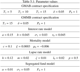
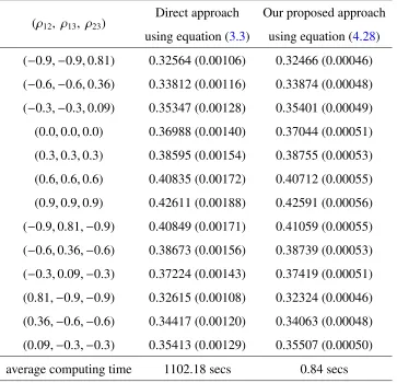
can be generated through equations (4.19)-(4.21) and equations (4.23)-(4.27). Our numerical results are based on 100,000 sample paths generated through the MC method in RStudio. A parallel-simulation technique is employed with the machine (i7-6820HK CPU @ 2.70 GHz, 8 Cores). The parameters used for equations (2.1), (2.3), (2.4) and (3.2) are depicted inTable 5.1. In Table 5.2, we display the price of a GMAB based on a cohort aged 50 at t = 0 and assuming a GMAB’s maturity at age 65, with the first and second renewals at ages 55 and 60, respectively. The codes for the results inTable 5.2are given inAppendix C.
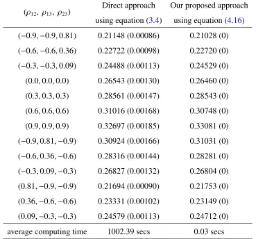
The prices of a GMMB based on the same cohort with same 15-year maturity are given in Table 5.3. The codes for generating the values inTable 5.3can be found inAppendix D. Both GMAB and GMMB contracts are evaluated att = 0 (age 50), and a wide range of correlation valuesρ12,ρ13andρ23 are tested to see their influence on GMAB and GMMB prices.
direct approach for the GMAB and GMMB, respectively; this establishes the efficiency of our measure-change method. It can also be observed that under the same maturityT3 = 15 years
and correlation values (ρ12, ρ13, ρ23), the GMAB is more expensive than the GMMB; the price
difference is solely attributed to the cost of the additional renewal options embedded in the GMAB contract.
Table 5.1: Parameter values GMAB contract specification
T1 = 5 T2 =10 T3 =15 δ=0.05 P0 =1
GMMB contract specification
T3 =15 δ =0.05 P0 =1
Interest rate model
a=0.15 b= 0.045 σ1 =0.03 r0= 0.045
Mortality model
c=0.1 ξ =0.0003 µ0 =−0.006
Lapse rate model
h=0.12 m=0.02 ζ =0.01 l0 =0.02 p= 0.5
Segregated fund model
Table 5.2: GMAB prices calculated using equations (3.3) and (4.28)
(ρ12, ρ13, ρ23)
Direct approach using equation (3.3)
Our proposed approach using equation (4.28) (−0.9,−0.9,0.81) 0.32564 (0.00106) 0.32466 (0.00046) (−0.6,−0.6,0.36) 0.33812 (0.00116) 0.33874 (0.00048) (−0.3,−0.3,0.09) 0.35347 (0.00128) 0.35401 (0.00049) (0.0,0.0,0.0) 0.36988 (0.00140) 0.37044 (0.00051) (0.3,0.3,0.3) 0.38595 (0.00154) 0.38755 (0.00053) (0.6,0.6,0.6) 0.40835 (0.00172) 0.40712 (0.00055) (0.9,0.9,0.9) 0.42611 (0.00188) 0.42591 (0.00056) (−0.9,0.81,−0.9) 0.40849 (0.00171) 0.41059 (0.00055) (−0.6,0.36,−0.6) 0.38673 (0.00156) 0.38739 (0.00053) (−0.3,0.09,−0.3) 0.37224 (0.00143) 0.37419 (0.00051) (0.81,−0.9,−0.9) 0.32615 (0.00108) 0.32324 (0.00046) (0.36,−0.6,−0.6) 0.34417 (0.00120) 0.34063 (0.00048) (0.09,−0.3,−0.3) 0.35413 (0.00129) 0.35507 (0.00050)
Table 5.3: GMMB prices calculated utilising equations (3.4) and (4.16)
(ρ12, ρ13, ρ23)
Direct approach using equation (3.4)
Our proposed approach using equation (4.16) (−0.9,−0.9,0.81) 0.21148 (0.00086) 0.21028 (0) (−0.6,−0.6,0.36) 0.22722 (0.00098) 0.22720 (0) (−0.3,−0.3,0.09) 0.24488 (0.00113) 0.24529 (0) (0.0,0.0,0.0) 0.26543 (0.00130) 0.26460 (0) (0.3,0.3,0.3) 0.28561 (0.00147) 0.28543 (0) (0.6,0.6,0.6) 0.31016 (0.00168) 0.30748 (0) (0.9,0.9,0.9) 0.32697 (0.00185) 0.33081 (0) (−0.9,0.81,−0.9) 0.30924 (0.00166) 0.31031 (0) (−0.6,0.36,−0.6) 0.28316 (0.00144) 0.28281 (0) (−0.3,0.09,−0.3) 0.26827 (0.00132) 0.26804 (0) (0.81,−0.9,−0.9) 0.21694 (0.00090) 0.21753 (0) (0.36,−0.6,−0.6) 0.23331 (0.00102) 0.23149 (0) (0.09,−0.3,−0.3) 0.24579 (0.00113) 0.24712 (0)
average computing time 1002.39 secs 0.03 secs
5.2
Price-sensitivity analyses
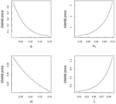
We perform a price-sensitivity analysis for the GMAB under some parameter-scenario settings. The results are exhibited inFigure 5.1andFigure 5.2and they reveal the impact of individual model parameters on the GMAB price. All plots are based on the correlations (ρ12, ρ13, ρ23)=
(0, 0, 0). Appendix E.1andAppendix E.2contain the algorithms in coming up withFigure 5.1 andFigure 5.2.
In the upper panel ofFigure 5.1, the parameterbis negatively related to the GMAB price. Note thatbis the mean-reverting level of the interest rate model, and a higher mean-reverting level implies a higher average of interest rate. Therefore, the higher the mean-reverting level, the greater the effect of the discounting factor exp−Rt
0 rudu
price. The right plot in the upper panel shows that the volatilityσ1 of the interest rate is
posi-tively related to the GMAB price. This outcome is consistent with the view that the higher the risk, the higher the associated potential yield. A similar pattern follows in the lower panel of Figure 5.1, wheremis the mean-reverting level of the lapse rate model andζis the correspond-ing volatility.
Figure 5.1: GMAB prices under different parameter values
b
GMAB pr
ice
0.05 0.10 0.15 0.20
0.1
0.2
0.3
0.4
0.5
m
GMAB pr
ice
0.05 0.10 0.15 0.20
0.20
0.25
0.30
σ1
GMAB pr
ice
0.02 0.04 0.06 0.08 0.10
1
2
3
ζ
GMAB pr
ice
0.01 0.03 0.05 0.07 0.09
0.5
0.7
0.9
Figure 5.2: GMAB prices under different parameter values
δ
GMAB pr
ice
0.02 0.04 0.06 0.08 0.10
0.2
0.4
0.6
0.8
1.0
1.2
σ2
GMAB pr
ice
0.01 0.07 0.13 0.19
0.4
0.5
0.6
InFigure 5.2, when the roll-up rateδincreases, the GMAB price increases; this is because a higher roll-up rate implies a higher guaranteed value, hence a higher payoffleading to a higher price. Another observation is that the GMAB price increases as the segregated fund’s volatility
σ2 increases. Again, this is consistent with the notion that the higher the uncertainty in the
performance of the segregated fund, the higher the potential return. Therefore, the GMAB price would have to increase enough to match the corresponding return level.
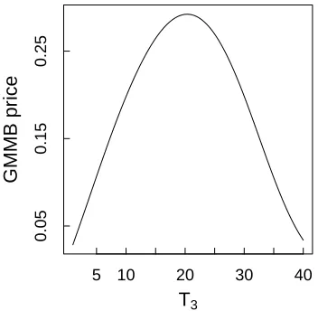
Figure 5.3: GMMB prices with various values of maturityT3
T3
GMMB pr
ice
5 10 20 30 40
0.05
0.15
0.25
pattern; seeFigure 5.3. This relationship pattern conveys that the price increases as the uncer-tainty increases, but after some time the discounting factor has the commanding effect, making the price to decline. Appendix E.3depicts the codes in generatingFigure 5.3.
InFigure 5.4, we display the GMAB prices, withT3 = 15 years, as a function of both T1
andT2, where the first renewal is assumed to be between year 2 and year 7 whilst the second
renewal is assumed to be between year 8 and year 13. The codes used to produce the results in Figure 5.4are shown inAppendix E.4.
Figure 5.4: GMAB prices versus varyingT1andT2
T1
2 3
4 5
6 7
T2
8 9 10
11 12 13
GMAB pr
ice
Conclusion
Actuarial practice needs a valuation approach that is sophisticated to capture the salient features of the underlying variables yet it must be easily implementable and adaptable to industry’s pric-ing platform. This research responds to this need and constructs a framework whose flexibility could extend to the pricing of other contracts with investment guarantees.
More specifically, we developed an integrated framework for the valuation of a GMAB, where three interrelated risk factors (i.e., interest, mortality, and lapse rates were considered). The change of measure technique was employed to obtain an explicit solution for the pure en-dowment, and therefore aiding the evaluation of risk-neutral conditional expectation for pric-ing. In particular, we utilised the forward measure and the survival measure to decompose the pure endowment into the product of the bond price, likelihood of survival, and lapsation probability. The streamlined valuation of a GMAB is finally achieved through the utility of the endowment-risk-adjusted measure. When the option to renew is not present, we success-fully derived an analytic solution for the so-called the GMMB contract. Numerical illustrations show that we created a computationally time-saving method with highly significant calculating speed and accuracy when compared to the benchmark chosen, which is the MC simulation method.
There are several possible natural avenues for future research. We may adopt the two-factor Hull-White model [10] instead of the Vasiˇcek model, which is noted for its ability to fit today’s term structure of interest rates. Note that the mortality model we adopted ignores the age pattern; so, it may be worthwile to consider the Cairns-Blake-Dowd model [3] in which both
[1] A. Bacinello, P. Millossovich, A. Olivieri, and E. Pitacco. Variable annuities: A unifying valuation approach. Insurance: Mathematics and Economics, 49(3):285–297, 2011.
[2] D. Bauer, A. Kling, and J. Russ. A universal pricing framework for guaranteed minimum benefits in variable annuities. ASTIN Bulletin, 38(2):621–651, 2008.
[3] D. Cairns, A.and Blake and K. Dowdd. A two-factor model for stochastic mortality with parameter uncertainty. Journal of Risk and Insurance, 73(4):687–718, 2006.
[4] J. Dhaene, A. Kukush, E. Luciano, W. Schoutens, and B. Stassen. On the (in-) depen-dence between financial and actuarial risks. Insurance: Mathematics and Economics, 52(3):522–531, 2013.
[5] D. Doyle and C. Groendyke. Using neural networks to price and hedge variable annuity guarantees. Risks, 7(1):1, 2019.
[6] G. Gan. Application of data clustering and machine learning in variable annuity valuation.
Insurance: Mathematics and Economics, 53(3):795–801, 2013.
[7] H. Gao, R. Mamon, and X. Liu. Pricing a guaranteed annuity option under correlated and regime-switching risk factors. European Actuarial Journal, 5(2):309–326, 2015.
[8] H. Gao, R. Mamon, X. Liu, and A. Tenyakov. Mortality modelling with regime-switching for the valuation of a guaranteed annuity option.Insurance: Mathematics and Economics, 63:108–120, 2015.
[9] M. Hardy. Investment Guarantees: Modeling and Risk management for equity-linked life insurance. John Wiley & Sons, 2003.
[10] J. Hull and A. White. Numerical procedures for implementing term structure models II: Two-factor models. Journal of Derivatives, 2(2):37–48, 1994.
[11] K. Ignatieva, A. Song, and J. Ziveyi. Pricing and hedging of guaranteed minimum bene-fits under regime-switching and stochastic mortality. Insurance: Mathematics and Eco-nomics, 70:286–300, 2016.
[12] LIMRA LOMA Secure Retirement Institute. Limra secure retirement institute: Fixed annuities continue to drive growth in first quarter 2019, 2019. Available online:
https://www.limra.com/en/newsroom/news-releases/2019/limra-secure-
retirement-institute-fixed-annuities-continue-to-drive-growth-in-first-quarter-2019/(accessed May 25, 2019).
[13] L. Jalen and R. Mamon. Parameter estimation in a regime-switching model with non-normal noise. InHidden Markov Models in Finance, pages 241–261. Springer, 2014.
[14] W. Kuo, C. Tsai, and W. Chen. An empirical study on the lapse rate: the cointegration approach. Journal of Risk and Insurance, 70(3):489–508, 2003.
[15] X. Liu, R. Mamon, and H. Gao. A comonotonicity-based valuation method for guaranteed annuity options. Journal of Computational and Applied Mathematics, 250:58–69, 2013.
[16] X. Liu, R. Mamon, and H. Gao. A generalized pricing framework addressing correlated mortality and interest risks: A change of probability measure approach. Stochastics, 86(4):594–608, 2014.
[17] E. Luciano and E. Vigna. Mortality risk via affine stochastic intensities: Calibration and empirical relevance. Belgian Actuarial Journal, 8:pages 5–16, 2008.
[18] R. Mamon. Three ways to solve for bond prices in the Vasiˇcek model. Advances in Decision Sciences, 8(1):1–14, 2004.
[20] Y. Zhao and R. Mamon. Annuity contract valuation under dependent risks.Japan Journal of Industrial and Applied Mathematics, pages 1–23, 2019.
[21] Y. Zhao, R. Mamon, and H. Gao. A two-decrement model for the valuation and risk measurement of a guaranteed annuity option. Econometrics and Statistics, 8:231–249, 2018.
Calculation details for the dynamics of
Λ
3
(
k
)
t
under
Q
This appendix provides calculation details to support the validity of equation (4.9). Using equation (4.6), we can rewriteΛ3(k)
t as
Λ3(k)
t B
Ht(k)Y
(k)
t M
(k)
t
M(0,Tk)
,
where
Ht(k)=e−
Rt
0rudue−A(t,Tk)rt+D(t,Tk),
Yt(k)=e−
Rt
0µudue−Ge(t,Tk)µt+He(t,Tk),
Mt(k)=e−
Rt
0ludue−I(t,Tk)lt−K(t,Tk)rt+J(t,Tk).
For any 0≤ s< t≤Tk, we have
EQ
h Ht(k)
Fs
i
=EQ
e−
Rt
0rudue−A(t,Tk)rt+D(t,Tk)
Fs
= EQ
e−
Rt
0ruduEQ
e−
RTk
t rudu
Ft Fs
=EQ
EQ
e−
Rt
0rudue−
RTk
t rudu
Ft Fs
= EQ
EQ
e−
RTk
0 rudu
Ft Fs
=EQ
e−
RTk
0 rudu
Fs
= e−
Rs
0 ruduEQ
e−
RTk
s rudu
Fs
=e−
Rs
0 rudue−A(s,Tk)rs+D(s,Tk) = H(k)
s .
So,Ht(k)is aQ-martingale, and the drift coefficient in theQdynamics ofH
(k)
t must be 0.
Using Itˆo’s Lemma, we have
dHt(k)=e
−Rt
0rudude−A(t,Tk)rt+D(t,Tk)+e−A(t,Tk)rt+D(t,Tk)de−
Rt
0rudu+de−A(t,Tk)rt+D(t,Tk)de−
Rt
0rudu
=−σ1A(t,Tk)H
(k)
t dW
1
t,
Similar arguments show that
dYt(k)=−ξGe(t,Tk)Y( k)
t
ρ12σ1A(t,Tk)dt+ρ12dWt1+
q
1−ρ2 12dW
2
t
and
dM(tk) =−M
(k)
t
ρ13ζI(t,Tk)+σ1K(t,Tk) σ1A(t,Tk)+ρ12ξGe(t,Tk)
+ζI(t,Tk)ρ
0
23ξGe(t,Tk)
q
1−ρ2 12
dt
−Mt(k)
ρ13ζI(t,Tk)+σK(t,Tk)
dWt1+ζI(t,Tk)ρ023dWt2 +ζI(t,Tk)
q
1−ρ2 13−ρ
02 23dW
3
t
.
By Itˆo’s Lemma, we have
dHt(k)Y
(k)
t =Y
(k)
t dH
(k)
t +H
(k)
t dY
(k)
t +dH
(k)
t dY
(k)
t
=−σ1A(t,Tk)H( k)
t Y
(k)
t dWt1 −ξGe(t,Tk)H(
k)
t Y
(k)
t
ρ12σ1A(t,Tk)dt+ρ12dWt1+
q
1−ρ2 12dW
2
t
+ρ12σ1A(t,Tk)ξGe(t,Tk)H
(k)
t Y
(k)
t dt =−Ht(k)Yt(k)
σ1A(t,Tk)+ρ12ξGe(t,Tk)
dWt1+ξGe(t,Tk)
q
1−ρ2 12dW
2
t
Furthermore,
dH(tk)Yt(k)Mt(k) =Mt(k)dHt(k)Yt(k)+Ht(k)Yt(k)dMt(k)+dHt(k)Yt(k)dMt(k)
=−Ht(k)Y
(k)
t M
(k)
t
σ1A(t,Tk)+ρ12ξGe(t,Tk)
dWt1+ξGe(t,Tk)
q
1−ρ2 12dW
2
t
−Ht(k)Yt(k)Mt(k)
ρ13ζI(t,Tk)+σ1K(t,Tk) σ1A(t,Tk)+ρ12ξGe(t,Tk)
+ρ0
23ζI(t,Tk)ξGe(t,Tk)
q
1−ρ2 12
dt
−Ht(k)Y
(k)
t M
(k)
t
ρ13ζI(t,Tk)+σK(t,Tk)
dWt1+ρ
0
23ζI(t,Tk)dWt2 +ζI(t,Tk)
q
1−ρ2 13−ρ
02 23dW
3
t
+Ht(k)Yt(k)Mt(k)
ρ13ζI(t,Tk)+σK(t,Tk) σ1A(t,Tk)+ρ12ξGe(t,Tk)
+ρ0
23ζI(t,Tk)ξGe(t,Tk)
q
1−ρ2 12
dt
=−Ht(k)Y
(k)
t M
(k)
t
σ1A(t,Tk)+ρ12ξGe(t,Tk)+ρ13ζI(t,Tk)+σ1K(t,Tk)
dWt1 +ξGe(t,Tk)
q
1−ρ2 12+ρ
0
23ζI(t,Tk)
dWt2+ζI(t,Tk)
q
1−ρ2 13−ρ
02 23dW
3
t
.
Thus, the dynamics ofΛ3(k)
t underQis given by
dΛ3(k)
t =−Λ
3(k)
t
σ1A(t,Tk)+ρ12ξGe(t,Tk)+ρ13ζI(t,Tk)+σ1K(t,Tk)
dWt1 +ξGe(t,Tk)
q
1−ρ2 12+ρ
0
23ζI(t,Tk)
dWt2+ζI(t,Tk)
q
1−ρ2 13−ρ
02 23dW
3
t
.
Calculation details for the covariances in
Chapter 4
This appendix provides the computational details to support the validity of equations (4.21), (4.25), (4.26) and (4.27).
We examine and evaluate one by one the four terms in equation (4.21).
CovQb2
h Y0(2),T
1,Y
(2)
T1,T2
i
=CovQb2
"Z T1
0
rt−α− 1 2σ
2 2
!
dt+σ2Wb
4(2)
T1 ,
Z T2
T1
rt−α− 1 2σ
2 2
!
dt+σ2
b W4(2)
T2 −Wb
4(2)
T1
#
=CovQb2
"Z T1
0
rtdt+σ2Wb
4(2)
T1 ,
Z T2
T1
rtdt+σ2
b W4(2)
T2 −Wb
4(2)
T1
#
=CovQb2
"Z T1
0
rtdt,
Z T2
T1
rtdt
#
+CovQb2
"Z T1
0
rtdt, σ2
b W4(2)
T2 −Wb
4(2)
T1
#
+CovQb2
" σ2Wb
4(2)
T1 ,
Z T2
T1
rtdt
#
+CovQb2
h σ2Wb
4(2)
T1 , σ2
b W4(2)
T2 −Wb
4(2)
T1
i .
Using equation (4.11), the first term can be expressed as
CovQb2
"Z T1
0
rtdt,
Z T2
T1
rtdt
#
=CovQb2
" σ1
Z T1
0
Z u
0
e−aueasdWb
1(2)
s du, σ1
Z T2
T1
Z u
0
e−aueasdWb
1(2)
s du
#
=CovQb2
" σ1
Z T1
0
1−e−a(T1−s)
a !
dWb
1(2)
s , σ1
e−aT1 −e−aT2
a
! Z T1
0
easdWb
1(2)
s
+σ1
Z T2
T1
1−e−a(T2−s)
a !
dWb
1(2)
s
#
=σ2 1
e−aT1 −e−aT2
a !
CovQb2
"Z T1
0
1−e−a(T1−s)
a !
dWb
1(2)
s ,
Z T1
0
easdWb
1(2)
s
#
=σ2 1
e−aT1 −e−aT2
a
! Z T1
0
1−e−a(T1−s)
a !
easds
=σ21
a2
e−aT1 −e−aT2
Z T1
0
eas−e−aT1e2asds
=σ21
a2
e−aT1 −e−aT2 1
ae
as− 1 2ae
−aT1e2as
!
s=T1
s=0
=σ21
2a3
e−aT1 −e−aT2 eaT1 +e−aT1 −2.
Moreover, the second term can be expressed as
CovQb2
"Z T1
0
rtdt, σ2
b W4(2)
T2 −Wb
4(2)
T1
#
=CovQb2
" σ1
Z T1
0
Z u
0
e−aueasdWb
1(2)
s du, σ2
b W4(2)
T2 −Wb
4(2)
T1
#
=CovQb2
" σ1
Z T1
0
1−e−a(T1−s)
a !
dWb
1(2)
s , σ2
b W4(2)
T2 −Wb
4(2)
T1
#
=0.
Futhermore, the third term can be expressed as
CovQb2
" σ2Wb
4(2)
T1 ,
Z T2
T1
rtdt
#
=CovQb2
" σ2Wb
4(2)
T1 , σ1
Z T2
T1
Z u
0
e−aueasdWb
1(2)
s du
#
=CovQb2
" σ2Wb
4(2)
T1 , σ1
e−aT1 −e−aT2
a
! Z T1
0
easdWb
1(2)
s
+σ1
Z T2
T1
1−e−a(T2−s)
a !
dWb
1(2)
s
#
=0.
Finally, the last term can be expressed as
CovQb2
h σ2Wb
4(2)
T1 , σ2
b W4(2)
T2 −Wb
4(2)
T1
i
= 0.
Therefore we have
CovQb2
h Y0(2),T
1,Y
(2)
T1,T2
i
= σ21
2a3
as desired.
Similar arguments show that
CovQb3
h Y0(3),T
1,Y
(3)
T1,T2
i
= σ21
2a3
e−aT1 −e−aT2 eaT1 +e−aT1 −2,
CovQb3
h Y0(3),T
1,Y
(3)
T2,T3
i
= σ21
2a3
e−aT2 −e−aT3 eaT1 +e−aT1 −2,
and
CovQb3
h YT(3)
1,T2,Y
(3)
T2,T3
i
= σ21
2a3
e−aT2 −e−aT3 eaT2 +e−aT2 −eaT1 −e−aT1.
Codes for GMAB evaluation
This appendix provides the R codes used to produce the results inTable 5.2.
C.1
Codes for the direct approach in the GMAB evaluation
1 # S e t t h e p a r a m e t e r v a l u e s
2 a=0 . 1 5 3 b=0 . 0 4 5 4 s i g m a 1=0 . 0 3 5 r 0=0 . 0 4 5 6 c=0 . 1 7 x i=0 . 0 0 0 3 8 u0=0 . 0 0 6 9 h=0 . 1 2 10 m=0 . 0 2 11 z e t a=0 . 0 1 12 p=0 . 5 13 l 0=0 . 0 2 14 s i g m a 2=0 . 0 5