A study of pairing computation for curves with embedding
degree 15
Nadia El Mrabet1, Nicolas Guillermin2, and Sorina Ionica3 1
LIRMM, Montpellier 2
DGA, Rennes 3
Universit´e de Versailles Saint-Quentin-en-Yvelines, 45 avenue des ´Etats-Unis, 78035 Versailles CEDEX, France
[email protected],[email protected]
Abstract. This paper presents the first study of pairing computation on curves with embedding degree 15. We compute the Ate and the twisted Ate pairing for a family of curves with parameter
ρ1.5 and embedding degree 15. We use a twist of degree 3 to perform most of the operations inFp orFp5. Furthermore, we present a new arithmetic for extension fields of degree 5. Our computations
show that these curves give very efficient implementations for pairing-based cryptography at high security levels.
Key-words:Pairing based cryptography, Pairing computation, Arithmetic, Interpolation, Elliptic Curves, Embedding degree, Security level.
1
Introduction
Pairings on elliptic curves were introduced by Andr´e Weil in 1948 in mathematics [24], but their utilization in cryptography is actually quite recent. They were first used for cryptanalytic purposes, i.e. attacking the discrete logarithm problem on supersingular elliptic curves [2], but nowadays they are also used as building blocks for new cryptographic protocols such as the tripartite Diffie-Hellman protocol [15], identity-based encryption [5], short signatures [6], and others. A pairing is a bilinear map e : G1×G2 →G3, where G1, G2 andG3 are groups of large prime orderr. Known pairings on elliptic curves, i.e. the Weil, Tate,
Eta and Ate pairings map to the multiplicative group of the minimal extension of the ground fieldFp
containing the r-th roots of unity. The degree of this extension is called the embedding degree with respect tor. The most efficient known method used for pairing computation is Miller’s algorithm, whose performance relies heavily on efficient arithmetic of this extension field. It follows that for efficient pairing computation we need curves with a rather small embedding degree.
On the other hand, latest research in efficient computation of pairings focused on the reduction of the loop length in Miller’s algorithm. It was proven [23][13] that on most known families of ordinary curves, the complexity of Miller’s algorithm isO(ϕ(1k)log2(r)), wherekis the embedding degree andϕis Euler’s totient function. Consequently, for a fixed level of security and therefore a fixed bit length ofr, pairing computation might turn out to be faster on curves with embedding degrees such that the integerϕ(k) is large. Moreover, in practice we are looking for curves for which the following valueρ=log2(p)
log2(r) is as small
as possible, in order to save bandwidth during the calculation.
In this paper, we give the first efficient pairing computation for curves of embedding degree 15. We show that existing constructions of families of curves of degree 15 and j-invariant 0 present multiple advantages. First of all, we show that pairing computation on these curves has loop length log2(r)
8 for the Ate pairing and log2(r)
2 for the twisted Ate pairing. Secondly, we show that by using twists of degree 3 we manage to perform most of the operations inFp orFp5. By making use of an interpolation technique, we
also improve the arithmetic ofFp5 in order to get better results.
Moreover, denominator computation and the final inversion can be avoided by making use of the twist. Our results show that by choosing the optimal arithmetic onFp5 and F
on curves of embedding degree 15 andρ= 1.5 is faster than on Barreto-Naehrig curves for high security levels, i.e. security levels of 192 and 256 bits. Our computations suggest that these curves might be the best choice one could make among known pairing-friendly families of curves for implementations at high security levels.
The remainder of this paper is organized as follows: Section 2 gives the definition and important properties of pairings. In Section 3 we establish the optimal computation of the pairing on curves with embedding degree 15. In Section 4 we describe an interpolation-based algorithm for multiplication over the fieldFp5. Finally, we conclude in Section 5 by giving a global evaluation of the number of operations
needed to compute the pairing and by comparing our results to performances obtained on Barreto-Naehrig curves, which are considered as standard at the time this paper was written.
2
Background on pairings
In this section we give a brief overview of the definitions of pairings on elliptic curves and of Miller’s algorithm [20] used in pairing computation. Letpbe a prime,E an elliptic curve defined overFp by the
Weierstrass equation y2 =x3+ax+b and r a prime factor of #(E(F
p)). Suppose r2 does not divide
#(E(Fp)) and let k be the embedding degree with respect to r, i.e. the smallest integer such that r
dividespk−1. We denote by P
∞ the point at infinity of the elliptic curve.
Definition 1. A pairing is a bilinear and non degenerate function:
e:G1×G2→G3
(P, Q)→e(P, Q)
where G1 and G2 are subgroups of order r on the elliptic curve and G3 is generally µr, the subgroup
of the r-th roots of unity in Fpk. In general, in cryptographic applications, we take G1 =E(Fp)[r] and
G2⊂E(Fpk)[r], where we denote byE(K)[r] the subgroup ofK-rational points of orderrof the elliptic curveE. We also denoteE[r] the subgroup of points of orderrdefined over the algebraic closure ofFp.
Let P ∈ G1, Q ∈ G2. The goal of Miller’s algorithm is to first construct a rational function fs,P
associated to the pointP and to some integersand to secondly evaluate this function at the pointQ(in fact at a divisor associated to this point). The functionfs,P is such that the divisor associated to it is:
div(fs,P) =s(P)−(sP)−(s−1)(P∞).
Suppose we want to compute the sum ofiP and jP. Takeh1 the line going throughiP and jP andh2 the vertical line through (i+j)P. Miller’s idea was to make use of the following relation
fi+j,P =fi,Pfj,Ph1
h2, (1)
in order to compute fs,P iteratively. Moreover, Miller’s algorithm uses the double-and-add method to
computefs,P in log2(s) operations.
The Tate pairing The Tate pairing, denoted eT ate, is defined by: G1×G27→G3
(P, Q)7→eT ate(P, Q) =fr,P(Q).
Here, the function fr,P is normalized, i.e. (ur0fr,P)(P∞) = 1 for ur0 someFp-rational uniformizer at
P∞. This pairing is only defined up to a representative of (Fpk)r. In order to obtain a unique value we raise it to the power pk−1
r , obtaining anr-th root of unity that we call the reduced Tate pairing
ˆ
eT ate(P, Q) =fr,P(Q)
Ate pairing Let πp be the Frobenius over the elliptic curve:πp : E →E, such that for P = (xP, yP)
πp(P) = (xpP, y p
P). The trace of the Frobenius is denoted byt. LetT =t−1,G1:=E[r]∩Ker(πq −[1])
andG2:=E[r]∩Ker(πq−[q]). Then for two pointsP ∈G1andQ∈G2, the Ate pairing is given by:
eate(Q, P) =fT,Q(P)(p
k−1)/r
It was shown in [14] that the Ate pairing is actually a power of the reduced Tate pairing.
Twisted Ate pairing We begin with the following definition.
Definition 2. Let E, E′
be elliptic curves over Fp. Then E′ is called a twist of degree d if there exists an isomorphismφd:E′ →E defined over Fpd anddis minimal.
Suppose now thatE admits a twist E′
defined overFpk/d of degree d, withd|k. We setm= gcd(k, d) ande=k/m. We considerG1 andG2 as above. Then forP ∈G1, Q∈G2 we get [14]:
etwisted(P, Q) =fTe,P(Q)(p k−1)/r
,
The twisted Ate pairing is also a power of the reduced Tate pairing. For curves with small trace of the Frobenius, it is clear that the Ate and twisted Ate pairings should be preferred to the Tate pairing, as the loop in Miller’s algorithm will be shorter. Other variants of twisted Ate pairing were obtained in [19] replacingTewith Tie, for anyi∈Z. All these variants were given in order to find the smallest possible
λdetermining the length of the loop in Miller’s algorithm. Hess and Vercauteren exploit these ideas in [13] and [23], respectively, by making use of lattices.
Optimal pairing Considersan integer andh=Pd
i=0hixi∈Z[x] withh(s)≡0 mod r. LetR∈E(Fqk) andfs,h,R the function whose divisor is
(fs,h,R) = d
X
i=0
hi((siR)−(P∞))
We denote||h||1=Pdi=0|hi|.
Theorem 1. Lets be any primitive root of unity modulor2 andnan integer dividing #Aut(E). Then
atwist
s,h :G1×G2→µr
(P, Q)→(fs,h,P(Q))(q
k−1)/r
.
defines a bilinear pairing which is non-degenerate if and only ifh(s)6≡0 modr2. The relation with the
Tate pairing is
atwist
s,h (P, Q) =t(P, Q)h(s)/r.
There exists an efficiently computable h ∈ Z with h(s) ≡ 0 modr, deg(h) ≤ ϕ(n)−1 and ||h||1 =
O(r1/ϕ(n)) such that the above pairings are non-degenerate. TheO-constant depends only on n.
Security aspect The security of a pairing based cryptosystem relies on two parameters: the bit length ofr, log2rand the bit size of the extension fieldklog2p. These parameters have to be chosen large enough to ensure that the discrete logarithm problem will be hard in both the subgroup of points of orderrof the curve and the multiplicative group of the finite fieldFpk. The fastest known attack on finite field is the in-dex calculus method, whose complexity isO(Lr(13)), whereLr(13) = exp ((32/9)(1/3)(logr)
1
3log(log(r)) 2 3)
Table 1.Level of security in bit
AES security bitsize ofrbitsize ofpk
80 160 1024
128 256 3072
192 384 7680
256 512 15360
on elliptic curves DLP is the Pollard-ρ method, whose complexity isO(√r) [9, Chap. 17]. As a conse-quence, while the security level will increase, the bound onklog2(p) is expected to grow faster than the bound on log2(r). Following NIST recommendations [1], Table 1 gives optimal bitsizes ofr and pk for different security levels.
On the other hand, in practice we are looking for curves for which the following value
ρ= logp logr
is as small as possible, in order to save bandwith during the calculation. This is due to the fact that for a fixed level of security, efficient implementation of the pairing depends on the size of the ground field, i.e. on the size ofp. So taking greaterkis a better solution than increasing the bit length ofp.
3
Optimal pairing for
k
= 15
A first method that could be used in order to build curves withk= 15 is the Cocks-Pinch method [8]. This method generates curves with arbitraryr and ρ∼2. Duan and all. [11] showed that by using the Brezing-Weng method we can actually do better. They generated a family of curves withj-invariant 0, embedding degree 15 andρ∼1.5. This family is given by the following polynomials:
p= 1/3x12−2/3x11+ 1/3x10+ 1/3x7−2/3x6+ 1/3x5+ 1/3x2+ 1/3x+ 1/3
r=x8−x7+x5−x4+x3−x+ 1
t=x+ 1.
The remainder of this paper will present efficient computation of pairings on this family of curves. To emphasize the performance of our suggestion, we compare our results to those resulting from efficient implementation of pairings on Barreto-Naehrig curves [4]. We briefly remind that these are curves of embedding degree 12 andj-invariant 0, given by the following parametrization:
p= 36x4+ 36x3+ 24x2+ 6x+ 1
r= 36x4+ 36x3+ 18x2+ 6x+ 1
t= 6x2+ 1.
These curves are preferred in cryptographic applications because they have the ρ ∼ 1 and most operations during the pairing computation are done in Fp or Fp2, thanks to the existence of a twist of
degree 6.
3.1 Twists of degree 3
Let E be an elliptic curve ofj-invariant 0, defined over Fp. Suppose its equation is y2 = x3+b, with
b∈Fp. ConsiderEover the extension fieldFpk/3. Then it admits a cubic twistE′of equationy2=x3+b
withD not a cubic residueD∈Fqk/3. The morphism
Φ3:E ′
→E:Φ3(x, y) = (xD1/3, yD1/2) maps points inE′
(Fpk/3) to points in E(Fpk). In particular, asr|#E′, we may chooseQ, the generator of G2, as the image of anr order point under this morphism : Q =Φ3(Q′
), with Q′ ∈ E′
(F
pk/3). So
Q = (D1/3x, D1/2y), with x, y ∈ F
pk/3. As we will see later, for k = 15 this will imply that most
operations in pairing computation onG1×G2 (orG2×G1) are to be done inFp orFp5.
3.2 Optimal pairing fork= 15
We can easily see that for the family of curves withk = 15 described above, the length of the Miller’s loop for the twisted Ate pairing is 58log2r. We will show that the complexity of the computation of the optimal pairing for this family is O(log2r
2 ). Indeed, we apply theorem 1 with n = 3 and compute the following polynomial using function field LLL ([21]):
h15(x, t) = (x3−x2+ 1)t−x4+x3−x+ 1 We compute
div (fs,h,P) = ((x3−x2+ 1)(sP)−((x3−x2+ 1)sP)−(x3−x2)(P∞)) + ((−x4+x3−x+ 1)(P)
−((−x4+x3−x+ 1)P)−(−x4+x3−x)(P∞)) + ((x3−x2+ 1)tP) +((−x4+x3−x+ 1)P)−2(P∞) = div (f
x3−x2+1,sP) + div (f−x4+x3−x+1,P) + divv(x3−x2+1)tP
Now it was shown in [14] thatG1=E[r]∩Ker(ζ3◦πp5−[p5]) andG2=E[r]∩Ker(ζ3◦πp5 −[1]) and
that fT5,ζ 3◦π5
p(P)◦ζ3◦π 5
p =fT5,P. We conclude that the optimal twisted Ate pairing for this family of
curves is given by the formula:
(fp
5
x3−x2+1,P(Q)f−x4+x3−x+1,P(Q))
p15−1 r .
Note that the evaluation atQof the vertical linev(x3−x2+1)tP can actually be ignored because of the final
exponentiation. So we need to computefx,P(Q),fx2,P(Q),fx3,P(Q) andfx4,P(Q) as well the evaluation
at Q of the lines lx3
P,−x2
P, l−x4
,x3, l
(−x4+x3,−x). So we get a complexity of O(logr/2) for the pairing
computation. The twisted Ate pairing has loop length log2r for Barreto-Naehrig curves, as a search for the optimal pairing on these curves gives, for example,
h12(x, t) = (2x+ 6x2)∗t+ 1 + 2x So the complexity of Miller’s algorithm is log2r
2 . The Ate pairing fork= 15 is given byfx,Q(P), so the loop length islog8r, while the optimal Ate pairing computation for Barreto-Naehrig curves has complexity O(log4r), as shown in [23]. We have also verified with MAGMA that our formulas give bilinear non-degenerated pairings.
3.3 Denominator elimination in pairing computation
We use an idea given in [18]. We observe that the expression of lineh2 in Equation ( 1) can be written as:
xT−xQ=
x3
T −x3Q
x2
T +xTxQ+x2Q
= y
2
T −yQ2
x2
T+xTxQ+x2Q
.
The element (y2
Q−y2T) is inFp5 and can be forgotten during the computation of the pairing, because of
the final exponentiation. Indeed,p5−1 is a divisor of p15
−1
r so multiplication by this term can be omitted.
Consequently at each iteration in Miller’s algorithm loop it suffices to multiply byx2
T+xTxQ+x2Q, instead
3.4 Operation count
Pairing computation on elliptic curves in Weierstrass form is usually performed in Jacobian coordinates (see [7], [3]), but we find that homogenous coordinates will give better results in our case. Our starting point is a suggestion for pairing computation in homogenous coordinates given in [10]. A point (X, Y, Z) in homogenous coordinates represents the affine point (X/Z, Y /Z) on the elliptic curve of affine equation
y=x3+c. Due to denominator elimination, the doubling step of the Miller loop becomes:
(2i)P ←2·(iP)
f2i,P ←fi,P2 h1(Q)ST(Q)
whereh1(Q) = 2Y ZyQ−3X2xQ+Y2−3cZ2 andST(Q) =Z2x2Q+XZxQ+X2. We compute (2i)P=
(X3, Y3, Z3) as
X3= 2XY(Y2−9Z2),
Y3= (Y −Z)(Y + 3Z)3−8Y3Z,
Z3= 2Y3Z.
We perform the operations in the following order:
A=Y2 B=Z2
C= (Y +Z)2−A−B Z3= 4A·C
E=X2
F = (X+Y)2−E−A X3=F·(A−9B)
Y3= (A−3B+C)·(A+ 9B+ 3C)−Z3.
We compute h1(Q)·ST(Q) as:
h1(Q)ST(Q) = (2Y ZyQ−3X2xQ+Y2−3cZ2)(Z2x2Q+XZxQ+X2) =
2X2Y ZyQ+ 2XY Z2xQyQ+ 2Y Z3x2QyQ−3X4xQ−3X3ZxQ2 −3X2Z2x3Q+
+(Y2−3cZ2)X2+ (Y2−3cZ2)XZx
Q+ (Y2−3cZ2)Z2x2Q
It follows that we need to perform the following operations:
G=B·C H =B·F
I =E2 K=(X+Z)
2−E−B 2
L=K2 M =F2
N = (A−3cB)·K O=E·K
P = (A−3cB)·B
This gives the following computation forh1(Q)ST(Q):
h1(Q)ST(Q) =F yQ+HxQyQ+Gx2QyQ−(3I−N)xQ−(3O−P)x2Q−3Lx3Q+M−3cL
We denote bySpn andMpnthe cost of a squaring and a multiplication, respectively, in the extension field of degreenofFp. We assume that the expressions ofxQ,x2
Q,yQ,xQyQ,x2QyQ are precomputed. As
with an element ofFp costs 5Mp. A count of the operations for the entire doubling step for the twisted
Ate pairing gives 9Sp+ 38Mp+Sp15 +Mp15. In the case of the Ate pairing doubling computation,
A, B, C, ...Lare elements of Fp5, so the operation count gives 30Mp+ 9Sp5 + 8Mp5 +Sp15 +Mp15. For
pairing computation on Barretto-Naehrig curves we only need to do the doubling of the point and compute
h1(Q). The operation count gives 5Sp+ 15Mp+Sp12+Mp12 for the doubling part of the twisted Ate
pairing and 4Mp+ 5Sp2+ 3Mp2+Sp12+Mp12 for the Ate pairing.
3.5 First comparison
We compare the complexity of pairing computation for the families of curves presented above, using Karatsuba and Toom Cook multiplication algorithms in the extension fields. The costs of multiplications are given in Table 2. We denote byAp the cost of an addition inFp. Table 3 gives recommended sizes of
randpfor different security levels. Using a classical arithmetic, we count the number of multiplications inFp needed for a Miller loop; we do not take into account the cost of the polynomial reduction one has
to perform.when multiplying two elements of the extension field. Indeed, Fp12 is usually constructed as
an extension ofFp2, which in turn is constructed asFp/(X2+ 1). The polynomials used to construct the
extension fields of degree 2 and 3 over this field then have constant termδinFp2; depending on the choice
of delta (not a square, nor a cube) the multiplication cost may vary. However in this paper we consider this influence negligeable. The resulting comparison for the Ate and twisted Ate pairings is given in Table 4.
Table 2.A performance evaluation: arithmetic ofFp15 versus arithmetic ofFp12
Mp2 Mp3 Mp5 Mp6 Mp12 Mp15
3Mp+ 4Ap5Mp+ 20Ap13Mp+ 58Ap15Mp+ 72Ap45Mp+ 180Ap65Mp+ 390Ap
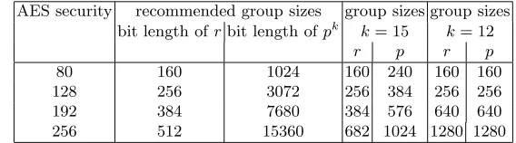
Table 3.A security evaluation: curves with embedding degree 15 versus Barreto-Naehrig curves
AES security recommended group sizes group sizes group sizes bit length ofrbit length ofpk k= 15 k= 12
r p r p
80 160 1024 160 240 160 160
128 256 3072 256 384 256 256
192 384 7680 384 576 640 640
256 512 15360 682 1024 1280 1280
Table 4.Pairing evaluation: curves with embedding degree 15 versus Barreto-Naehrig curves
Ate pairing Twisted Ate pairing Security level in bits k= 15 k= 12 k= 15 k= 12
It becomes clear that at 80 and 128 bits security levels Barreto-Naehrig curves give most efficient pair-ing computation. On the other hand, for 192 and 256 security levels, the family of curves with embeddpair-ing degree 15 and ρ 1.5 gives pairing computations faster than on Barreto-Naehrig curves. Moreover, note that Karatsuba is optimal for extensions of degree 2, so it seems quite natural to question these results. We propose in the next Section an improvement of the arithmetic onFp5 using the Newton interpolation
method to compute a multiplication between two elements ofFp5.
4
Finite field arithmetic
In cryptography, and more generally in arithmetic, we need an efficient polynomial multiplication. The optimization can be in time or elementary operations. Pairing Based Cryptography (PBC) follows the same rules as PBC involves polynomial computations. Indeed A andB ∈ Fpk are represented as poly-nomials of degree (k−1) in γ, with γ a root in Fpk of a polynomial of degree k, irreducible over Fp. If possible, the irreducible polynomial is chosen to be Xk−β, with β ∈F
p. In the case of k = 5, this
condition is true for every primepsuch thatp≡1mod(5) [17, Theorem 3.75].
Theorem 2. Let Fp be a finite field and β be an element ofFp such that β is not a k-th power of an element ofFp. Then the polynomial Xk−β is irreducible over Fp.
In extensions of degree 2 or 3 the Karatsuba and Toom Cook multiplications are the most efficient. For higher degree extension, one can use tower field extensions [16] and apply Karatsuba and Toom Cook [25], or multiplication by interpolation [25]. Generally, interpolation methods have an important drawback: they increase the number of additions during a multiplication. We present a multiplication by Newton interpolation which, despite the extra additions, improves the global complexity of a multiplication in
Fp5 when compared to the Karatsuba multiplication.
4.1 Interpolation
We denote byA(X) =a0+a1X+. . .+ak−1Xk−1,B(X) =b0+b1X+. . .+bk−1Xk−1 the polynomials obtained by substitutingγ byX in the expressions ofAand B in Fpk. Multiplications by interpolation follow these steps:
• Find 2k−1 different values inFp {α0, α1, . . . , α2k−2}.
• Evaluate the polynomialsA(X) andB(X) at these 2k−1 values:A(α0), . . . , A(α2k−2), B(α0), . . . , B(α0). • ComputeC(X) =A(X)×B(X) at these 2k−1 valuesC(αi) =A(αi)B(αi).
• InterpolateC(X) polynomial of degree 2k−2 either with Lagrange or Newton interpolation.
We describe our method of multiplication using the Newton interpolation, which is more efficient for our purpose than Lagrange interpolation [25]. The use of FFT [25] is not interesting in our case. Indeed, during a FFT multiplication, we have to multiply by roots of unity. As we do not have any control on the characteristicpwe work with, the roots of unity do not necessarily have a sparse representation, even after recoding. It follows that multiplications by these roots are expensive. Furthermore, the choice of values of interpolation in Section 4.3 is not interesting for the FFT method. Last but not least, FFT is very interesting for extensions of large even degree, which is not the case for the finite fieldFp5. Consequently,
we focused on the Newton interpolation.
4.2 Newton interpolation
c′
0= C(α0)
c′
1= (C(α1)−c′0)(α1−1α0)
c′ 2=
(C(α2)−c′0)(α2−1α0)−c
′ 1
1 (α2−α1)
..
. = ...
The reconstruction ofC(X) is done by
C(X) =c′ 0+c
′
1(X−α0) +c′2(X−α0)(X−α1) +. . .+c2′k−2(X−α0)(X−α1). . .(X−α2k−2). It can be computed using the Horner scheme:
C(X) =c′
0+ (X−α0) [c′1+ (X−α1) (c′2+ (X−α2)h. . .i)]
So, complexity in term of operation of Newton interpolation is the sum of the complexities of these different operations:
1. the evaluations inαi ofA(X) etB(X)
2. the 2k−1 multiplications inFp (A(αi)×B(αi) )
3. computation of thec′
i
4. the Horner scheme to find the expression ofC(X) =A(X)×B(X) of degree 2k−1.
4.3 Simplifying operations of the Newton interpolation for k= 5
We consider thatk= 5, the 2k−1 = 9 chosen values for the interpolation are:
α0= 0, α1= 1, α2=−1, α3= 2, α4=−2, α5= 4, α6=−4, α7= 3, α8=∞.
We choose those value in order to minimize the number of additions and divisions by the differences of theαi during the interpolation.
In the following section, we denoteAp an addition,Mp a multiplication, andSp a square inFp.
Complexity of the evaluations inαi ofAand B First of all, we have to evaluateA(X) andB(X) at theαi’s. With the chosen values, evaluations of A(X) andB(X) are done using only additions and
shifts inFp. Indeed, a product by a power of 2 is composed of shifts in binary base, so in order to evaluate
A(X) at 2j, we compute the products a
i×(2j)i, and perform the additionsPk
−1
i=0ai(2j)i using a FFT
scheme.
Writing down 3 = 2 + 1, the evaluation in 3 is only composed of shifts and additions too. Indeed, powers of 3 can be decomposed as sum of powers of 2: 32= 23+ 1, 33= 25−22−1 et 34= 26+ 24+ 1.
Adding the different costs, evaluations ofA(X) andB(X) have a complexity of 50Ap.
Once we have the evaluations, we have to compute the multiplications A(αi)×B(αi) which are
obtained with 9Mp. The complexity of the steps 1 and 2 altogether is then 50Ap+ 9Mp.
Complexity of the computations of c′
j In order to compute the coefficientsc ′
j during a Newton
interpolation, one has to compute exact divisions by the differences of the αi ∈ Fp. We call an exact
division a division where the dividend is a multiple of the divisor. Among all the differences of the αi
Table 5.The problematic differences
α3−α2= 3 α4−α1 =−3 α5−α1= 3 α5−α2= 5
α5−α4= 6 α6−α1 =−5 α6−α2=−3 α6−α3=−6
α7−α0= 3 α7−α4= 5 α7−α6= 7
We describe here the method to execute the exact division. We want to divide δ, a multiple of 3, by 3, i.e.δverifies thatδ= 3×σand we want to findσ. This equality can be rewritten asσ=δ−2×σ. If
δ=Xiδi2i andσ=
X
iσi2i we can findσbit after bit beginning with the less significant bit. Indeed,
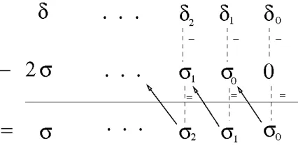
σ=δ−2×σgivesσ0=δ0. Thus we can findσ1 as the result of the subtraction:δ1δ0−σ00 =σ1σ0. By extrapolation we findσ1, and thenσ2 and the following as explained in Figure 1.
Fig. 1.Scheme for the division by 3 in one addition
Consequently, an exact division by 3 is theoretically done with exactly one subtraction in Fp. The
same scheme can be applied to an exact division by 5. Indeed, forχ= 5×κ(i. e. knowingχwe want to findκ), we just have to consider thatκ=χ−4×κ. Then the exact division by 5 has the complexity of a subtraction.
The cost of an exact division by 7 is the same as the one of an addition inFp, provided that we find
first the negative of the result. We knowµ= 7×ν, and we want to findν. We transform the equation: −ν =µ−8×ν. So first we find−ν with an addition inFp, and then it is quite easy to findν.
We consider that the complexity of a subtraction is equivalent to the complexity of an addition, which is an upper bound for a subtraction. The implementation aspect is considered in Section 4.4. As a consequence, the exact divisions by 3, 5 and 7 can be computed with only an addition. The eleven divisions by these values have a complexity of 11Ap.
In order to have the complexity of the computation of the c′
j, we must take into consideration the
subtractions. There are 28 subtractions in the formulas of thec′
j.
Thus, the complexity of the computation of the c′
j is 39Ap.
Complexity of the polynomial interpolation We use the Horner scheme to find the expression of the product polynomialC=A×B. The Horner scheme consists in writing and computing:
C(X) = ((((c′
8(X−α7) +c′7)(X−α6) +c′6)(X−α5) +c′5). . .+c1′)(X−α1) +c′0. We begin to compute from the inside (the parenthesis (c′
8(X −α7) +c′7)) to the outside, i.e. we compute ((c′
the construction of the polynomial using the Horner scheme is composed of multiplications of the i-th parenthesis byα7−iand additions. With the chosen values ofα′is the Horner scheme is composed only of
additions.
So the complexity of the polynomial expression with the Horner scheme is 29Ap.
4.4 Results and implementation aspects
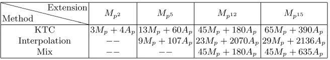
We have described the multiplication by interpolation for an extension of degree 5 of a finite field. Table 6 gives the complexity of multiplications with several methods: the classical Karatsuba and Toom Cook multiplications (KTC), the interpolation multiplication. The third line of Table 6 (Mix) gives the cost of a multiplication inFp15 using a tower of extension fields. We use our Newton multiplication in Fp5 and
the Toom Cook method for the extension field of degree 3 overFp5.
Table 6.Complexity of different method of multiplication
X X
X X
X X
X X
X
Method
Extension
Mp2 Mp5 Mp12 Mp15
KTC 3Mp+ 4Ap13Mp+ 60Ap 45Mp+ 180Ap 65Mp+ 390Ap Interpolation −− 9Mp+ 107Ap23Mp+ 2070Ap29Mp+ 2136Ap
Mix −− −− 45Mp+ 180Ap 45Mp+ 635Ap
Using these results, it becomes clear that it is better to use a multiplication by interpolation instead of a multiplication using Karatsuba Toom Cook for extension fields of degree 5. We save 4 multiplications in Fp using interpolation whereas we add 47 additions. The extra cost due to these additions is not
as important as the cost to compute 4 multiplications in Fp. Indeed, the complexity of a Karatsuba
multiplication inFp is
5Nlog2(3)A
w+Nlog2(3)Mw,
whereN is the number of bytes of the considered integers, and whereAw andMwrepresent an addition
and a multiplication of a word.
We designed the exact division by 3 on a Stratix 2 FPGA (speed grade 3). The result of this implemen-tation is that the division we present can be done in the same time as an addition. We compute the exact division of an integer of size 240 bits in 13.9 ns, which is an acceptable latency to be executed in one clock cycle. In comparaison, on the same FPGA the ripple-carry adder, which takes benefit of carry propagation mechanism, achieves a 14.2 ns latency on an integer addition of the same length. Thus our hyptothesis in Section 4.3 is verified and the complexity we give is true.
On the contrary, for extensions of degree 12 and 15, using an interpolation to compute a multiplication is not so interesting. The additional cost of the additions is huge in comparison to the saved multiplica-tions. The interpolation method is very interesting for an extension of degree 5, because we can choose the value of interpolation such that the number of additions does not increase too much in relation with the saved multiplications. Table 7 gives the comparison of a pairing computation considering the number of multiplications and additions at different security levels.
Table 7 gives our final comparison. We used our improved arithmetic for an extension of degree 5 to compute a multiplication inFp5. We compare our result to the complexity of the pairing computation on
Barreto-Naehrig curves.
Note that we have only counted the number of operations in Fp, but the base field has different
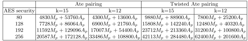
Table 7. A performance evaluation of the Ate pairing computation: curves with embedding degree 15 versus Barreto-Naehrig curves
Ate pairing Twisted Ate pairing
AES security k=15 k=12 k=15 k=12
80 4830Mp+ 53760Ap 4300Mp+ 13600Ap 9880Mp+ 88900Ap 7800Mp+ 25200Ap 128 7728Mp+ 86064Ap 6900Mp+ 21760Ap 15808Mp+ 142240Ap 12480Mp+ 40320Ap 192 11592Mp+ 129096Ap 17007Mp+ 54400Ap 23712Mp+ 213360Ap31200Mp+ 100800Ap 256 20587Mp+ 172128Ap33486Mp+ 108800Ap42113Mp+ 284480Ap62400Mp+ 201600Ap
levels, pairing computation is more efficient on curves with embedding degree 15 and ρ∼ 1.5 than on Barreto-Naehrig curves (note that at these security levels the bitlength ofpis shorter fork= 15). We evaluated the cost of final exponentiation using the techniques proposed in [22] and our computations showed that this operation has approximatively the same cost for curves withk= 15 andρ∼1.5 and for Barretto-Naehrig curves at 256-bits security level (about 960Sp15 fork = 15 and 940Sp12 fork = 12).
However, for lower security levels the final exponentiation will be more expensive for the case k = 15 because it depends on the value ofρ∼1.5. Further work needs to be done to find families of curves of embedding degree 15 with betterρvalue if we want to make this case interesting for lower security levels.
5
Conclusion
In this paper, we give efficient pairing computation for curves of embedding degree 15. We show that existing constructions of families of curves of degree 15 and j-invariant 0 present multiple advantages. First of all, we show that pairing computation on these curves has loop length log8r for the Ate pairing and log2r for the twisted Ate pairing. Secondly, we show that by using twists of degree 3 we manage to perform most of the operations inFporFp5. Moreover, denominator computation and the final inversion
can be avoided by making use of twists. By using of an interpolation technique, we also improve the arithmetic ofFp5 in order to get better results.
References
1. Recommendations for Key Management, 2007. Special Publication 800-57 Part 1.
2. S. Vanstone A. Menezes, T. Okamoto. Reducing elliptic curve logarithms in a finite field.IEEE Transactions
on Information Theory, 39(5):1639–1646, 1993.
3. C. Arne, T. Lange, M. Naehrig, and C. Ritzenhaler. Faster Pairing Computation, 2009. http://eprint.iacr.org/2009/155.
4. P. Barreto and M. Naehrig. Pairing-friendly elliptic curves of prime order. InSelected Areas in Cryptography - SAC 2005, volume 3897 ofLecture Notes in Computer Science, pages 319 –331. Springer, 2006.
5. D. Boneh and M. K. Franklin. Identity-based encryption from the Weil pairing. In Joe Kilian, editor,Advances
in Cryptology – CRYPTO 2001, volume 2139 ofLecture Notes in Computer Science, pages 213–229. Springer
Verlag, 2001.
6. D. Boneh, B. Lynn, and H. Shacham. Short signatures from the Weil pairing. In Colin Boyd, editor,
Advances in Cryptology – ASIACRYPT 2001, volume 2248 of Lecture Notes in Computer Science, pages
514–532. Springer Verlag, 2001.
7. Sanjit Chatterjee, Palash Sarkar, and Rana Barua. Efficient computation of tate pairing in projective coor-dinate over general characteristic fields, 2004.
8. C. Cocks and R.G.E. Pinch. Indentity-based cryptosystems based on the Weil pairing. unplublished manuscript, 2001.
10. C. Costello, H. Hisil, J.M.G. Nieto, and K.K.H. Wong. Faster Pairings on Special Weierstrass Curves. Pairing 2009, 2009. to appear.
11. P. Duan, S. Cui, and C.W. Chan. Special polynomial families for generating more suitable elliptic curves for pairing-based cryptosystems. In The 5th WSEAS International Conference on Electronics, Hardware,
Wireless Optimal Communications, 2005.
12. R. Granger, A.J. Holt, D. Page, N.P. Smart, and F. Vercauteren. Function field sieve in characteristic three.
InApplied Cryptography and Network Security) 2004, volume 3076 ofLectures Notes in Computer Science,
pages 223–234. Springer, 2004.
13. F. Hess. Pairing Lattices. In Steven Galbraith and Kenny Peterson, editors,Pairing 2008, volume 5209 of
Lectures Notes in Computer Science, pages 18–38, 2008.
14. F. Hess, N. P. Smart, and F. Vercauteren. The Eta Pairing Revisited. IEEE Transactions on Information Theory, 52:4595–4602, 2006.
15. A. Joux. A one round protocol for tripartite Diffie-Hellman.Journal of Cryptology, 17(4):263–276, September 2004.
16. Neal Koblitz and Alfred Menezes. Pairing-based cryptography at high security levels. In Nigel P. Smart, editor,IMA Int. Conf., volume 3796 ofLectures Notes in Computer Science, pages 13–36, 2005.
17. R. Lidl and H. Niederreiter. Finite Fields. 2nd ed., Cambridge University Press, 1997.
18. X. Lin, C. Zhao, F. Zhang, and Y. Wang. Computing the Ate Pairing on Elliptic Curves with Embedding Degree k = 9. IEICE Transactions, 91-A(9):2387–2393, 2008.
19. Seiichi Matsuda, Naoki Kanayama, Florian Hess, and Eiji Okamoto. Optimised versions of the ate and twisted ate pairings. In the Eleventh IMA International Conference on Cryptography and Coding, pages 302–312. Springer-Verlag, 2007.
20. Victor S. Miller. The Weil pairing, and its efficient calculation.Journal of Cryptology, 17(4):235–261, Septem-ber 2004.
21. S. Paulus. Lattice basis reduction in function fields. In Joe Buhler, editor,ANTS III, volume 1423 ofLectures
Notes in Computer Science, pages 567–575, 1998.
22. M. Scott, N. Benger, M. Charlemagne, L.J.D. Perez, and E.J. Kachisa. On the final exponentiation for calculating pairings on ordinary elliptic curves. to appear in Pairing 2009, 2009.
23. Frederik Vercauteren. Optimal Pairings, 2008. http://eprint.iacr.org/2008/096. 24. Andr´e Weil. Courbes alg´ebriques et vari´et´es ab´eliennes (in french. Hermann, 1948.