On a Rigorous Proof of the Existence of Complex Waves
in a Dielectric Waveguide of Circular Cross Section
Yury Shestopalov1, * and Ekaterina Kuzmina2
Abstract—Existence of symmetric complex waves in a dielectric rod (DR) — a dielectric waveguide of circular cross section — is proved by analyzing functional properties of the dispersion equations (DEs) using the theory of functions of several complex variables and validating the existence of complex roots of DE. A closed-form iteration procedure for calculating the roots in the complex domain supplied with efficient choice of initial approximation is proposed. Numerical modeling is performed with the help of a parameter-differentiation method applied to the analytical and numerical solution of DEs.
1. INTRODUCTION
A dielectric waveguide of circular cross section, a dielectric rod (DR), is a basic structure in the broad family of open waveguides. Many works are devoted to the analysis of complex waves in open dielectric waveguides; one may refer in this respect to [1–3] to mention a few, and to other monographs on dielectric waveguides and textbooks on electromagnetics. Elements of the mathematical theory of complex waves can be found, e.g., in [4–6]. However, rigorous mathematical proof of the existence of complex waves in a DR remains, to the best of our knowledge, one of fundamental unsolved problems of the theory of electromagnetic wave propagation in open waveguides. This statement may be indirectly validated by considering, e.g., a recent publication [7] that contains a comprehensive reference list on this topic. Typical approaches developed by many authors searching for complex waves are reduced to numerical solution in the complex domain of dispersion equations (DEs) associated with symmetric waves in a DR (in many cases using commercial solvers) or incorrect replacement of the initial DEs by simplified equations employing various approximations or asymptotic expansions (see, e.g., [8] and [9]). Such numerical-analytical investigations are not supported by mathematically correct proofs of the existence and analysis of distribution of the complex wave spectra.
Let us briefly analyze in this respect the approach [9] employing the Davidenko’s method. In [9] the authors consider a DE for the DR complex waves without specifying the domain of the functions entering the DE (and analysis of all their singularities and branch points) and constructing analytical continuation of these multi-valued functions to the complex domain of the chosen spectral parameter (longitudinal wavenumber). The latter is necessary in order to use the Davidenko’s method because in this method the analyticity of the functions involved in the DE is applied and directly the Cauchy-Riemann conditions. Next, the problem is reduced to an ordinary differential equation (without validation of the equivalence of such a transition) where the initial conditions are not set which does not allow one to proceed with its solution. Any independent proofs of the existence of the DE roots are absent, as well as a description of the domain in the complex plane where the roots are situated. This circumstances complicate efficient computations and make doubtful the obtained numerical results.
Received 1 May 2018, Accepted 5 October 2018, Scheduled 25 October 2018
* Corresponding author: Yury Shestopalov ([email protected]).
1 Faculty of Engineering and Sustainable Development, University of G¨avle, G¨avle, Sweden. 2 Moscow Technological University
138 Shestopalov and Kuzmina
Such a situation may be explained by the absence of solid mathematical background which did not allow for completing rigorous proof of the existence of complex waves.
The aim of this study is to fill these gaps in the theory, at least partially, and complement the conventional methods of analysis of complex waves with the missing proofs and mathematical validation of the numerical procedures.
Determination of complex waves requires
(i) correct mathematical statements of the corresponding eigenvalue problems supplied with the conditions at infinity that allows for analysis and correct classification of complex waves;
(ii) obtaining functional equations for eigenvalues (DEs), proofs of the existence of complex zeros of the functions involved in DEs, and finding complex zeros of these DEs specified in terms of functions of several complex variables.
Such comprehensive studies have never been finalized as far as rigorous proof of the existence and correct determination of complex waves in a DR are concerned. This circumstance has become a driving force for us to complete the proofs and make the corresponding mathematical methods available and open for scientific community.
It should be noted that in [10] and [11], the methods developed in [12] have been applied, and the existence has been proved as a countable spectrum of running waves in a broad family of inhomogenously filled shielded waveguides which contains infinitely manycomplex points. This recent finding provides a solid base for the conjecture that open dielectric waveguides also have complex waves, which is rigorously demonstrated in this study.
In this work, we prove the existence of symmetric complex waves in a dielectric waveguide of circular cross section, a DR, by developing the mathematical methods set forth in [13]. We investigate the distribution of complex roots of the DEs that describe symmetric complex waves in a DR using the results of [13] and [14] and the discovered similarity between complex-valued functions entering the DEs. An iteration procedure for calculating zeros in the complex domain is developed in a closed form. An efficient choice of initial approximations in this procedure is governed by a theoretical description of localization of the DE roots.
As a result of the analysis, we identify ‘surface’ and ‘pure’ complex waves in a DR. The former is a regular perturbation of standard real surface waves [15, 16] with real longitudinal wavenumbers, whereas the latter, being a phenomenon inherent to a DR, is not connected with any real surface wave. The existence of ‘surface’ complex waves in a Goubau line is proved in [17].
Rigorous analysis of the existence and distribution of complex roots of DEs has required deep mathematical investigations of the properties of multi-parameter functions involved in DEs as functions (mappings) of several complex variables that may lead to the occurrence of complex zeros. A basic question on the first step of this analysis is to identify and correctly describe complex zeros considered with respect to the problem parameters as multidimensional hyper-surfaces in appropriate spaces of variables. Complexity of this task is explained by the fact that the sought-for quantities have singularities that generally form singular hyper-surfaces in parameter spaces.
2. STATEMENTS
Consider the propagation of symmetric eigenwaves, described in terms of nontrivial solutions to homogeneous Maxwell’s equations, in a DR with a radius a. Longitudinal wavenumber ks of the
symmetric waves is determined as
ks2=
k20−β2, r > a, k02−β2, r < a
Here,βis the wave propagation constant (spectral parameter),is the permittivity of the homogeneous dielectric, andk0 is the free-space wavenumber. The symmetric (azimuthally-independent) waves have
the nonzero components
H = [0, H2(r, z),0], E= [E1(r, z),0, E3(r, z)], (1)
E1 = − iβ k2 s
dφ dre
−iβz, E
3 =φ(r)e−iβz, H2 =− iω
k2 s
dφ dre
whereφis a cylindrical function satisfying the Bessel equation:
Lφ≡ 1 r d dr rdφ dr
+ks2φ= 0. (3)
Determination of symmetric waves in a DR can be reduced to the following singular Sturm-Liouville boundary eigenvalue problems on the half-line with a discontinuous (piecewise constant) coefficient in the differential equation:
Lφ= 0, r >0, [φ]|r=a =
k2 s dφ dr r=a
= 0, (4)
φ∈C1[0,+∞) ∩C2(0, a)∩C2(a,+∞). (5) Problem in Eqs. (4), (5) must be complemented with the conditions at infinity which are considered below.
Supplying Eq. (4) with the conditions at infinity
φ(r)→0, r → ∞ (6)
gives rise to Sturm-Liouville boundary eigenvalue problems on the half-line describing symmetricsurface
waves in DR. The surface waves are described in terms of real-valued quantities; in particular, the boundary operators in Eq. (4) are defined (as real-valued functions of a real variableγ orλ=γ2) on a certain intervalI specified below. In [14] it is proved that the spectrum of surface waves may be empty, or they may consist of several (real) points located on this interval.
It should be noted that the results of the classical Sturm-Liouville theory concerning existence and distribution of the (real) spectrum are not applicable here. The corresponding proofs in [13] and [14] employ reduction of the boundary eigenvalue problem in Eq. (4) with condition of Eq. (6) to DEs and their analysis using parameter differentiation and the method of Cauchy problem.
Make the following designations:
γ = β
k0
, κ=k0a, x=κ
−γ2, u=κ√−1, w=u2−x2=κγ2−1. (7)
For surface waves, potential functionφ(r) can be represented, according to the conditions at infinity in Eq. (6), as
φ(r) =
⎧ ⎪ ⎨ ⎪ ⎩ AK0 r aw
, r > a,
BJ0
r
ax
, r < a.
(8)
Here, Jk(x), Yk(x), K0(x), and K1(x) denote, respectively, the Bessel and Neumann functions of the
order k= 0,1 and the McDonald functions.
The form of the solution in Eq. (8) atr > a is governed by an asymptotic representation at large |z|
K0(z) =CK0 e−z
√
z
1 +O
1 |z|
(9)
which provides the fulfillment of condition at infinity of Eq. (6).
To investigate complex symmetric waves complement in Eq. (4) with a condition at infinity which is to a certain extent more general than Eq. (6); namely, make use of a relation between the Hankel and Macdonald functions
Kn(z) = π
2i
n+1H(1)
n (iz), n= 0,1, (10)
and a simpler version of the Reichardt-Sveshnikov condition [12] and assume that
φ(r) =AH0(1)(rw˜), r > a,
˜
w= i
a
u2−x2=k 0
1−γ2,
140 Shestopalov and Kuzmina
which is to be added to statement in Eqs. (4), (5) so that representations of Eq. (8) are preserved. Here
γ may be complex quantity, and ˜w is the transverse wavenumber of the medium outside DR (vacuum). The resulting boundary value problem in Eqs. (4), (5), (11) constitutes a nonselfadjoint eigenvalue problem w.r.t. spectral parameter γ. Their eigenvalues, real or complex, specify symmetric waves in Eqs. (1), (2) having normalized propagation constant (longitudinal wavenumber) γ; these waves are called, respectively, real or complex.
3. DISPERSION EQUATION
By applying to Eq. (8) the conditions of continuity of φ and its derivative at the point where the coefficient is discontinuous, we obtain the desired DE in the form [14]
xJ0(x) J1(x)
=u2−x2H (1) 0 (i
√
u2−x2)
H1(1)(i√u2−x2), (12)
which will be considered in what follows w.r.t. new variable x(instead of β). Rewrite Eq. (12) as
Gd(x, u) =Fd(x), (13)
or
FD(x, u) = 0, FD(x, u)≡Gd(x, u)−Fd(x), (14)
where
Gd(x, u) = −w K0(w) K1(w)
, (15)
Fd(x) = xcotj(x), cotj(x) := J0(x) J1(x)
. (16)
One may call function cotj(x) thecylindrical cotangent, because it exhibits all basic properties of the trigonometric cotangent; namely, cotj(x) takes all real values on every interval (νm1, νm+11 ), cotj(x)>0,
x∈(νm1, νm0), and cotj(νmn) = 0, whereνmn, m= 0,1,2, . . ., are themth zeros of Bessel functionsJn(x)
(n= 0,1).
The existence of real symmetric surface waves is proved [14] by considering Equations (13) and (14) w.r.t. the (real) independent variable
x=κ2(−1)−w2=κ−γ2, x∈(0, κ√−1)
where≥1. Ifx∗∈(0, κ√−1) is a root of Eq. (14), then
γ∗ = − x∗ κ 2
∈(1,√) (17)
is the propagation constants of a real symmetric surface wave.
To prove the existence of roots of Equation (14), it is reasonable, following [14], to considerx=x(u) as an implicit function of the parameteru >0 defined by Equation (14) and prove then that this function exists for all u > u∗, where u∗ > ν01. Namely, using the properties of the cylindrical cotangent and functionGd(x, u), we can prove, in line with the results obtained in [14], that if
u=κ√−1> ν10, (18)
then there exists a root
x=x∗∈(ν10, ν11) (19)
of DE (14); if
u∈(ν10, ν11), (20)
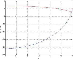
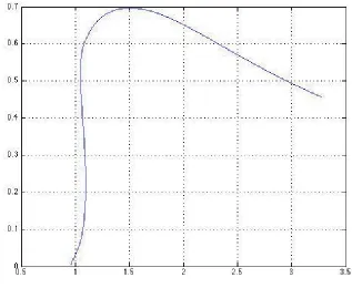
then Eq. (14) has only one root. Fig. 1 illustrates the rigorous proof in the case of Eq. (20) completed in [14].
Thus we arrive at the known result: there are at most finitely many symmetric surface waves propagating in a lossless ( = 0, > 1) DR and their normalized propagation constants γ ∈I0 =
Figure 1. Location of the first real zero of ˜FD at = 10, = 0 and κ = 1; the value of u=κ√−1 = 3∈(ν10, ν11) is marked by◦ and of the first zeroν10 = 2.4048 of J0(x) by ∗.
4. EXISTENCE OF COMPLEX WAVES
To investigate complex waves, consider the DE for surface waves in DR w.r.t. the complex variable
z=κ−γ2, whereγ is a complex quantity, in the form
˜
FD(z, u) = 0, F˜D(z, u)≡G˜d(z, u)−F˜d(z), (21)
where
˜
Gd(z, u) = −
1
wK(w), K(w) =
K1(w) K0(w)
, w=u2−z2, (22)
˜
Fd(z) =
1
zT(z), T(z) = tanj(z), tanj(z) := J1(z) J0(z)
. (23)
tanj(z) is a meromorphic function of z with a set of real poles that are zeros of the Bessel function
J0(z), and ˜Gd(z, u) is an analytical function in a bandB(u) :{z > u,0< z < U0}; the value of U0
is determined by the location of the zeros of Macdonald (and Hankel) function K0(ζ) situated closest
to the real axis ζ = 0.
4.1. Necessary Asymptotic Estimates
The following asymptotic estimates [18] hold for the Hankel functions at large values of|z|
Hn(1)(z) =
2
π
ei(z−π4)
√
z
l−1
k=0
ikak(n) zk +R
n l(z)
, (24)
|Rnl(z)| ≤ 2|al(n)| |z|l e
n−14|z|1
142 Shestopalov and Kuzmina
ak(n) =
(n−1)(n−32). . .(n−(2k−1)2)
k!8k , (26)
n = 0,1; 0<argz < π; l= 1,2, . . . . (27) Using relation in Eq. (10) between the Hankel and Macdonald functions and formulas (15) and (24)–(27) we can obtain the estimates at large values of |z| for function ˜Gd(z):
G˜d(z) = 1 ||
Cg1
|z|
1− u
2
2|z|2 +O
1 |z|4
×
1 +
l−1
k=1 ak(1)
wk +R 1 l(w)
1 +
l−1
k=1 ak(0)
wk +R 0 l(w)
≤ |1
| Cd
|z|. (28)
Applying similar estimates at infinity for the Bessel functions J0(z) and J1(z) it is easy to check
(taking into account that these functions have the same leading term
2
π
1 √
z in their asymptotic
expansions at infinity) that the cylindrical tangent tanj(z) = JJ1(z)
0(z) admits the uniform estimate
|tanj(z)| ≤Ctanj, z=y0 >0, |z| ≥x0>0, (29)
with a certain constant Ctanj.
Introduce the functions
g(z) = ˜FD(z) =g1(z) +g2(z),
g1(z) =
1
ztanj(z) =
1
z J1(z) J0(z) ,
g2(z) =
1
w K1(w) K0(w)
, w=u2−z2.
(30)
In view of the power series expansions of the analytical functionsJn(z),n= 0,1, in the vicinity of zero,
it is easy to check that
lim
z→0g1(z) =
1
2 (31)
and
|g1(z)| ≤Sg1 <1, |z| ≤z0 < ν10 = 2.4048, (32)
where, in line with Eq. (7), z=κ−γ2, and there is an ˆa
S such that
|tanj(z)| ≤δg1 if κ <ˆaS
for any (arbitrarily small)δg1 >0.
For the modified Bessel functions, in view of their power series expansions in the vicinity of zero, we have asymptotic representations
K0(z) =−ln z
2 +O(1), K1(z) = 1
z + z
2ln
z
2 +O(z). (33) Next
g2(w) =
1
1
w K1(w) K0(w)
= 1 1 w 1 w + w 2 ln w
2 +O(z) −lnw
2 +O(1)
,
so that g2(w) is unbounded in the vicinity of zero; namely, according to Eq. (7), w =
√
u2−x2 = κγ2−1, and there is an ˆa
L such that
|g2(w)|> Lg2 if κ <ˆaL (34)
for any (arbitrarily large) Lg2 >0.
4.2. Existence and Distribution of Complex Roots of DE
We prove existence and distribution of complex roots of the DE associated with symmetric complex waves in a DR using an approach developed in [13] and [14]. The possibility of applying this technique is based on the discovered similarity between complex-valued functions entering the DEs.
4.2.1. DE Analysis in the Complex Domain
To perform correct mathematical analysis of the existence and distribution of complex and real roots of the DE
g(z) = 0, g(z)≡F˜D(z) =g1(z) +g2(z), (35)
where functiong(z) is given by (30), which is equivalent to DEs in Eqs. (14) and (21) for, respectively, real and complex surface waves (see Appendix A), consider the functions of complex variables entering DE in Eq. (35) w.r.t. all the three problem parameters,
g = ˜g(z,d¯), (36)
¯
d = (κ, , ), =, = , (37)
or
g= ˆg(γ,d¯). (38)
In the latter case ˆg= ˆg(γ) is considered, for every fixed parameter vector ¯d, following the statement of the corresponding Sturm-Liouville problem in Eqs. (4), (11), at γ ∈ Λ, where Λ is the multi-sheet Riemann surface of the functionf(γ) = ln1−γ2.
The domain of ˆg(γ) is Λ excluding the sets of singular points
Γ0:
⎧ ⎨
⎩γ =γm(κ, ) =
− ν0 m κ 2
, m= 1,2, . . .
⎫ ⎬
⎭ (39)
where νm0, m = 0,1,2, . . . are zeros of the Bessel function J0(x) (singularities of cylindrical tangent
tanj(z), more precisely, simple real poles of its analytical continuation, a meromorphic function tanj(z)), and
ΓH :
⎧ ⎨
⎩γ=γk(κ, ) =
+
ζk0 κ
2
, k = 1,2, . . .
⎫ ⎬
⎭ (40)
whereζk0, k= 0,1,2, . . .are zeros of the Hankel function. Note that Γ0and ΓH are actually well-defined sets of three-dimensional hyper-surfaces if to consider them w.r.t. three real parameters κ, , .
Figure 2 exemplifies the parameter dependence showing, at= 10, ‘level curves’ of the first three hyper-surfaces γm(κ, , ) =
−(νm0
κ )2, m= 1,2,3, belonging to Γ
0; the curves γ
m(1, ) =γm(t) =
(t)−(ν0
m)2, m= 1,2,3, are parametrized by t= ∈[0,25]. We see that at
> p2, p= ν
0 1
κ , (41)
the initial point (γ(1,10,0), γ(1,10,0)) = (γ(1,10,0),0) of the curve γ1(1, ) =γ1(t) =
(t)−p2,
whereγ1(1,10,0) =γ1(0) =
10−p2 is on the real axis, and at
< p2, (42)
on the imaginary axis of the complex γ-plane (see Fig. 2). The same conditions
>p2 or <p2 (43)
144 Shestopalov and Kuzmina
Figure 2. Plots ofγm(κ, ) =γm(t) =
(t)−(ν0m
κ )2,m= 1 (red) and 2, 3 atκ= 1 and(t) = 10 +ti.
4.2.2. Surface Complex Waves
‘Surface complex waves’ have complex propagation constantsγm=γm(t) (complex eigenvalues of BVP
in Eqs. (4), (5), (11)) that constitute regular perturbation w.r.t. the parameter t = = of the propagation constants of real surface waves. The latter has real propagation constantsγm,0=γ(= 0),
where m= 1,2, . . . , N, γm,0 is determined as real roots of DE in Eq. (13), and their quantityN using
Eq. (18) from the condition
u=κ√−1> νN0. (44)
The existence of ‘surface complex waves’ is proved following [17] by the reduction to the Cauchy problem
dγm dt = ˜Φ
D
m(γm, t), γm(0) =γm,0,
˜
ΦDm(γm, t) =−
∂F˜D(γm, t) ∂t ∂F˜D(γm, t)
∂γm
, (45)
whereγm,0 ∈(1,√) is any solution of Equation (13) at = 0. The Cauchy problem in Equation (45)
is uniquely solvable under the condition
∂F˜D(γm,0,0)
∂γm
= 0, (46)
which is fulfilled becauseγm,0 is a simple zero of ˜FD(γ,0) and has a (locally unique) continuous solution γm =γm(t),t∈(0, T), satisfying the initial conditionγm(0) =γm,0,m= 1,2, . . ..
Sum up the results concerning the existence of ‘surface complex waves’: let (t) =+it,t≥0; then under modified condition of Eq. (44)
u=κ√−1> νN0, N = 1,2, . . . , >1, (47) there are N symmetric surface real (t = 0) or complex (t > 0) waves in a DR; propagation constants
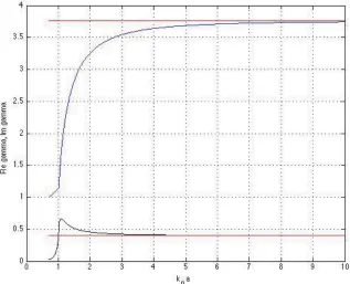
Figure 3. Imaginary (black) part of the first zero γ1 = γ1(κ) of ˜FD on the complex γ-plane at
= 20,28 and = 3 as κincreases from 0.65 to 10 and γ1(κ) merges with
√
(red lines).
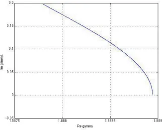
Figure 4. The first complex zeroγ1( ) of ˜FD (corresponding to a principal surface complex wave) on
146 Shestopalov and Kuzmina
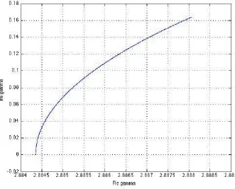
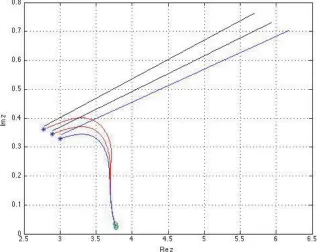
Figure 5. The first complex zero γ1( ) of ˜FD on the complex γ-plane at κ = 1.1 and = 20
(u =κ√19) as decreases from 1 to 0; the values calculated in the complex domain at = 0 are
z1= 3.7594 + 0.0000i andγ1= 2.8844 + 0.0000i.
real surface waves ‘starting’ from the real axis on the complex γ-plane at t = = 0, as depicted in Figs. 4–6 in smaller scale and smaller parameter interval t∈[0,1] and in Figs. 7 and 8 in larger scale and larger parameter intervalst∈[0,7.34], [0,17.04].
Figures 9–11 illustrate local transformation vs κ of the first zero z1 = z1(κ) of ˜FD and the
correspondingγ1=γ1(κ) of the principal complex surface wave on the complexz- orγ-planes. Figs. 12–
14 exemplify regularity of complex surface waves considered vs κ in relation to real surface waves: the behavior of the real and imaginary parts of complex waves is similar to their real counterparts. The curves in Figs. 12–14 resemble the known results obtained numerically by other authors (see, e.g., [7]). The spectrum of (proper) surface complex waves is located in a band 0 ≤ γ < sκ, where sκ, ≤ s0 < 1 in a broad interval of variation of t = , up to t = 20; for example, on Fig. 8, s0<0.25. Next, the length of the curvesγ(t) (in other words, the degree of variation of γ w.r.t. t) for
surface complex waves is by an order of magnitude smaller than that for pure complex waves; this is clearly seen if to compare the curves on Figs. 4–8 with those on Figs. 18 and 23.
4.2.3. ‘Pure’ Complex Waves
Before to prove the existence of ‘pure’ complex waves formulate the conditions that provide the absence of zeros of the function g(z) defined by Eq. (30).
Comparing Eqs. (34) and (32) we see that for any (complex) there is an ˆa= ˆa() such that the equation
g(z) ≡g1(z) +g2(z) = 0 (48)
has no roots in a ballB0 : |z|< z0
if κ <ˆa. (49)
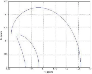
Figure 6. The first complex zero γ1( ) of ˜FD on the complex γ-plane at κ = 1 and = 10 as increases from 0 to 7.34; the values calculated in the complex domain at = 0 and 7.34 are, respectively,γ1(0) = 1.0815 + 0.0000i and γ1(7.34) = 0.9879 + 0.1225i.
Figure 7. Dynamics of the first complex zeros γ1( ) of ˜FD on the complex γ-plane at κ = 1 and
148 Shestopalov and Kuzmina
Figure 8. Dynamics of the first complex zeros γ1( ) of ˜FD on the complex γ-plane at κ = 1 and
= 8,10,13 (left, central and right curves) as increases from 0 to 17.04. The stars and small circles correspond, respectively, to the parameter values = 0 and 17.04.
Figure 9. The first zero γ1 = γ1(κ) of ˜FD on the complex γ-plane at = 12 and = 3 as γ(κ)
Figure 10. The first zeroz1=z1(κ) of ˜FD on the complexz-plane at = 12 and = 3 (red curve)
asκ decreases from 3.1055 to 0.6165 andz1(κ) merges with u=u(κ) =κ
√
−1 (blue line).
Figure 11. The first zeros z1 =z1(κ) of ˜FD on the complex z-plane at = 12,13,14 (lower curve,
blue) and = 3 as κ decreases from 1.7 to 0.83 and z1(κ) merge with u = u(κ) = κ
√
150 Shestopalov and Kuzmina
Figure 12. Real (blue) and imaginary (black) parts of the first zeroγ1=γ1(κ) of ˜FD on the complex γ-plane at= 14 and = 3 asκincreases from 0.7 to 10 andγ1(κ) and γ1(κ) merge, respectively,
with√= 3.763 and √= 0.398 (red lines).
Figure 13. Real part of the first three zeros γm=γ1(κ) m= 1,2,3, of ˜FD on the complex γ-plane at
Figure 14. Imaginary part of the first three zeros γm = γ1(κ) m = 1,2,3, of ˜FD on the complex γ-plane at = 24 and = 0.1 asκ increases from 1.9 to 10 and γ1(κ) merges with √(red line).
such that Equation (48) has no roots in a ball B0
if |u|<U .ˆ (50)
Prove first the existence of complex zeros of g(z) outside a vicinity of the origin of the complex
z-plane.
Functiong(z) does not vanish at zeros νm0,m= 0,1,2, . . . of the Bessel functionJ0; therefore these
points may be excluded from the analysis.
We will prove the existence and analyze the distribution of complex zeros of function g(z) using the well-known distribution of the set of (real) zeros of the Bessel functions J0(x) and J1(x) and the
resulting properties of the cylindrical tangent tanj(z) = JJ1(z)
0(z):
- J0(x) andJ1(x) have each a countable sequence of positive simple zeros;
- the distance |νn
m+1−νmn|between two neighboring zeros tends toπ asx→ ∞;
- there are numbersrn>0 such thatrn= minm|νm+1n −νmn|,m= 0,1,2, . . .,n= 0,1;
- zeros νm1 (ν01 = 0) and singularities νm0 of tanj = JJ1(z)
0(z) alternate: ν 1
m ∈ (νm0, νm+10 ) and
mink=m,m+1|νk0−νm1|<0.5r0,m= 0,1,2, . . ..
Consequently, the distances between zeros and singularities of the ‘almost-periodic’ cylindrical tangent tanj(z) are not constant; however, these quantities are bounded from below (and from above).
Let Γm = {z : |z−νm1|= r}, m = 1,2, . . ., r < 0.5r0. Inside every circle Γm function g1(z) has
exactly one zero of multiplicity one at the pointzm=νm1, m >0. According to the conditionr < r0 the
poles ofg1(z) (at the points νm0, m >0) are situated outside the circles. In view of the aforementioned
properties of tanj we see that there is an M0>0 such that M0 = const = min
z∈Γm, m=1,2,...|tanj(z)|, (51) C0M0
152 Shestopalov and Kuzmina
Here, function g1(z) is continuous on Γm; therefore the constantM0 >0 exists and does not depend on m. For function g2(z) estimate of Eq. (28) is valid
max
z∈Γm|g2(z)| ≤
1 ||
Cd
|z|. (53)
Now, we can prove the existence of ‘pure’ complex waves.
Statement E. Assume that the following conditionsE are fulfilled: if
is fixed and = 0, there is an ˆAL such that
κ >AˆL, (54)
or
κ is fixed, there is anε(0)>0 such that
|| ≥ε(0) >1, = 0, (55) or
there is anU(0)>0 such that
u=κ√−1≥U(0). (56)
Then, functiong(z) has exactly one (complex) zero of multiplicity one at a point zm∗ inside Γm.
Note first that for a fixedu, if |1z| → 0 then |w1| → 0 because|w|=|z||(uz)2−1|; more precisely,
if |1z| < δthen |w1| < CδwhereC is a constant independent ofz (in other words,wand zhave the same asymptotic when |z| → ∞). In view of this, inequalities of Eqs. (34), (52), and (53), and estimate of Eq. (29) all conditions of the Rouche’s theorem for
(a) the ballBm ={z: |z−νm1|< r} bounded by circle Γm and
(b) functionsg1(z),g2(z), andg=g1+g2 are fulfilled under condition (55):
|g1(z)|>|g2(z)|, z∈Γm. (57)
Next,g1(z) has exactly one zero of multiplicity one at a pointzm =νm1 ∈Bm. Therefore, function g(z) also has exactly one (complex) zero of multiplicity one at a certain point zm∗ inside Γm (see
Fig. 15 and the table of zeros zD,m, m= 1,2, . . .5, of ˜FD in Appendix B).
Figures 16 and 17 show position of the first complex zeros z1∗ = z1∗( ) of ˜FD on the complex z-plane (and Fig. 18 similar curves on the complex γ-plane) at κ = 1 and = 8,10,13 in relation to u =u( ) = κ√−1. We see that in a large interval of variation of ∈ [0,7.34] the transverse wavenumbers of the first (principal) complex surface wave stay in close proximity (shown in Fig. 15) of the first zero ν11 = 3.8317 of J1(x) and inside a band ν10 < z < ν11, where ν10 = 2.4048 is the
first zero of J0(x) as demonstrated in Figs. 19 and 20. Fig. 18 demonstrates the same property on
the complexγ-plane showing plots of the first three complex zerosγm(t) that virtually merge with the
curvesγ1m(κ, ) =γm(t) =
(t)−(νm1
κ )2 (m= 1,2,3) calculated atκ= 1 and(t) = 10 +ti,t∈(2,5).
Under condition of Eq. (56), there are infinitely many zeros ofg(z) in the right half-plane Rez≥0, and the uniform estimate is valid
g(zk∗) = 0, |zk∗−zk| ≤L,κ (58)
for a certain constantL,κ, as illustrated by Figs. 15 and 16.
Figure 22 shows typical distributions of the first zeros of ˜FD on the complex γ-plane at different
values of . Fig. 24 demonstrates zeros of ˜FD on the complex γ-plane vs at different values of . Figs. 25 and 26 show the first zeros of ˜FD on the complex γ-plane vs κ at different values of .
Figs. 27–29 illustrate the behavior of zerosγm( ) of ˜FD on the complex γ-plane w.r.t. (decreasing
or increasing) as these curves terminate at γ= 0.
Figure 15. Position of the three complex zeros z∗m =zD,m of g(z) = ˜FD(z) located in the vicinities
of the zeros zm = νm1 = 10.1735,13.3237,16.4706 (m = 3,4,5) of tanj(z) = J1(z)
J0(z) (crosses) calculated
by the Newton method in the complex domain at κ = 1 and = 10 + 10i (red stars) and= 10 + 6i
(small circles above stars); small circles on the real line denote the polesνm0 = 8.6537,11.7915,14.9309 of tanj(z) alternating with its zeros; closed curves are circles Γm of the radiusr <0.5 mink=2,3(νk+10 −νk0)
centered at zm,m= 3,4,5.
Figure 16. Position of the first complex zerosz1( ) of ˜FD on the complexz-plane in a circular vicinity
(black circle) of the first zero ν11 = 3.8317 of J1(x) (cross) at k0a= 1 and = 8,10,13 (left, central
154 Shestopalov and Kuzmina
Figure 17. The magnitude of the first complex zeros |z1( )| of ˜FD and |u( )| = κ|
√
−1| (green curves) vs at κ = 1 and = 8,10,13 (lower, middle, and upper curves). The first two zeros
ν1,20 = 2.4048,5.5201 ofJ0(x) and the first zeroν11 = 3.8317 of J1(x) are shown by red lines.
Figure 18. Plots of the first three complex zerosγm(t) and the curvesγm1(κ, ) =γm(t) =
(t)−(νm1 κ )2
Figure 19. The first zerosz1 =z1(κ) of ˜FD on the complexz-plane at= 12 and = 3−0.2(k−1), k = 1,2, . . .8 (lower curve: = 1.4) as κ decreases from 2 to 0.8; crosses denote the values
u=u(κ= 0.8) and vertical lines the first zerosν1n of Bessel functions Jn(x) (n= 0,1).
Figure 20. The first zerosz1 =z1(κ) of ˜FD on the complexz-plane at= 14 and = 3−0.1(k−1), k = 1,2, . . .30 (lower curve: = 0.1) as κ decreases from 2 to 0.8; crosses denote the values
156 Shestopalov and Kuzmina
Figure 21. The first zero γ1 =γ1(κ) of ˜FD on the complex γ-plane at = 12 +k, k= 1,2, . . . ,10,
and = 3 asγ(κ) approaches the real axis when κdecreases from 3.1055 to 0.83, ◦and ∗correspond, respectively, toκ= 3.1055 and 0.83 and the red curve to = 21.
(1) Propagation constants (longitudinal wavenumbers) of symmetric complex waves are eigenvalues of problem in Eqs. (4), (11) and roots of DE in Eq. (35).
(2) The imaginary and real axes of the principal (‘proper’) sheet Λ0 of the Riemann surface Λ of the
functionf(γ) = ln1−γ2 specified by w≥0 do not contain eigenvalues of problem in Eqs. (4),
Figure 23. The first 11 zeros of ˜FD on the complex γ-plane at 11 different values of = 2 + (10−
0.5(k−1))i,k= 1, . . . ,11.
158 Shestopalov and Kuzmina
Figure 25. The first zero of ˜FD on the complex γ-plane vs κ = 0.4−2.4 at = 5, = 12 (lower
curve) and = 1 (upper curve).
Figure 27. The first zeros of ˜FD on the complex γ-plane as they approach the imaginary axis at = 5, = 12 (κ decreases from 0.48 to 0.336, upper curve) and = 10 (κ decreases from 0.4 to 0.35, lower curve).
(11) except the intervalI0 = (1,
√
).
(3) Assume that conditions of Eqs. (54), (55), or (56) are fulfilled. Then there is a countable set of symmetric complex waves of the DR having the (normalized complex) propagation constants (longitudinal wavenumbers)
γm =
−
z
D,m κ
2
(59)
for themth-order complex symmetric wave corresponding to themth zerozD,mof Eq. (21) situated
in the vicinity of themth root νm1,m= 1,2, . . ., of the Bessel function J1.
(4) Assume that conditions of Eqs. (49) or (50) are fulfilled. Then DE in Eq. (35) has no roots, and consequently there are no symmetric complex waves.
The mathematical proof using Rouche’s theorem is of great practical significance. Indeed, this result guarantees the presence of one complex zero of the function g(z) = ˜FD(z) in the ball Bm = {z : |z−νm1| < r} of sufficiently small radius. Thus possibility is ensured to choose an initial
guess located in Bm that provides stable computations of the DE roots by the Newton method in
the complex domain and rapid convergence of iterations: usually, five to ten iterations provide up to 16 correct decimals in the calculated complex zeros (see the tables in Appendix C). On the other hand, (rapidly) convergent Newton iterations immediately validate the theoretical results concerning the existence of zeros.
A closed-form iteration procedure based on the Newton method in the complex domain is described in Appendix B.
4.3. On Dynamics of Complex Waves
160 Shestopalov and Kuzmina
Figure 28. The first zeros of ˜FD on the complex z-plane at= 12 and = 5 (lowest curve), 4,3,2
(highest curve);κ increases from 0.7 to 1.5.
Beginning from Fig. 24, all subsequent figures demonstrate actually different cases of wave dynamics determined and visualized for different parameter sets.
Specifically, we have studied wave dynamics analyzing (complex) roots of DE, or zeros z∗D of the functiong= ˆg(γ,d¯) defined by DE in Eq. (35) (eigenvalues of the Sturm-Liouville problem in Eqs. (4), (11)) as hyper-surfaces
zD∗ =zD∗( ¯d) (60)
defined explicitly by Eq. (35) using representation of Eq. (36).
Local existence of hyper-surfaces in Eq. (60) can be proved by formulating the corresponding initial value problems and the use of the Cauchy-Kowalevski theorem in the real or complex domain concerning the existence of solutions to a system of two or three differential equations in three dimensions.
When one parameter is varied, the wave dynamics is investigated by the reduction to the Cauchy problems of the type in Eq. (45) where the right-hand side of the initial condition is a function of the remaining parameters. The corresponding parameter curves solving Eq. (45) are locally one-to-one with respect to the quantity parametrizing the curve, e.g.,t= in Eq. (45). Generally, the behavior of the corresponding parameter curves solving Eq. (45) outside the proximity of the point where the initial condition is stated may be complicated.
Simpler versions of this method are when only one parameter from set ¯d is taken as a variable quantity and the remaining are fixed. Such an approach has been applied (without complete mathematical justification) in a majority of works devoted to the study of real and complex waves in dielectric waveguides. We use this technique below, investigating the occurrence of zeros of ˆg(γ,d¯) org(z,d¯) as implicitly defined functionszD∗ =z∗D( ),zD∗ =z∗D(), or zD∗ =zD∗(κ) and the like.
Figure 29. The first zeros of ˜FD on the complexγ-plane at= 12 and = 5 (lowest curve), 4, 3,
2 (highest curve);κ increases from 0.7 to 1.5.
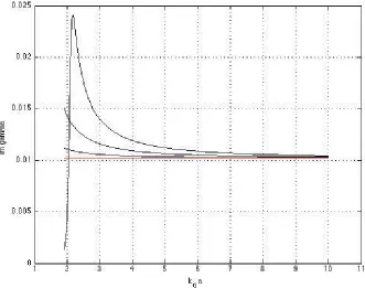
a special study. Fig. 3 exemplifies irregular dynamics in the form of a sharp local maximum in the dependence of the imaginary part of the higher-order surface complex waves on the relative radius κ
of DR. Another type of irregular wave dynamics is illustrated by Figs. 19–21 demonstrating the curves
z1=z1(κ) of the first zeros of ˜FD on the complexz-plane and the correspondingγ1(κ) on the complex γ-plane at several values of asκ decreases from 2 to 0.8; one can see that all the curves merge at a certain point, which is actually a singular point of the dependence on parameterκ.
In this work, we limit the analysis to several particular cases of regular dynamics explained in the text and illustrated by Figs. 4–11 and 25–29. A particular case of such a regular complex wave dynamics results from introduction of a small imaginary part of the permittivity that creates a regular perturbation of the spectrum of surface waves in DR shown partially in Figs. 4–11.
5. CONCLUSION
We have proved the existence of symmetric complex waves in a dielectric waveguide of circular cross section and have determined the location of the corresponding set of complex roots of DE.
It has been shown that the determination of the spectrum of symmetric complex waves is reduced to nonselfadjoint singular Sturm-Liouville boundary eigenvalue problems on the half-line where the conditions at infinity is formulated so that all types of complex waves may be taken into account.
In order to achieve the goals of the study, we have performed comprehensive mathematical investigations of the properties of the functions of several complex variables entering DEs. We have identified and correctly described complex roots of DE as implicit functions and multidimensional hyper-surfaces considered with respect to the problem parameters.
Two general families of complex waves have been identified, conditionally called ‘surface’ and ‘pure’ complex waves depending on the character of the dependence of their longitudinal wavenumbers on the problem parameters, location on the complex plane, and behavior at infinity.
162 Shestopalov and Kuzmina
introduction of small losses. In this study, the existence of complex surface waves is established numerically and requires further theoretical analysis.
We have performed numerical modeling using a parameter-differentiation method and analytical and numerical solution to the corresponding Cauchy problems applied to the analytical and numerical solution of DEs.
Numerical investigation of complex waves performed in this study does not require any solvers or standard data codes. The iteration procedure of calculating complex roots of DE in the complex domain providing fast convergence is written in the compact closed form. The efficient choice of initial approximation is validated by the determination of domains of localization of complex zeros as circles of small radii centered at zeros of Bessel functions.
The dynamics of waves in the complex domain has been investigated. We have shown in particular that introducing a small imaginary part of the permittivity creates a regular perturbation of the spectrum of surface waves in DR.
The methods developed in this study and the results obtained will be used as a mathematical background to determine complex wave spectra for broader families of open dielectric waveguides including Goubau lines and multi-layered fibers.
ACKNOWLEDGMENT
The author would like to thank Yury Smirnov for valuable ideas concerning the proof of the existence of complex zeros of DEs and acknowledge support of the Swedish Institute, project Largescale.
APPENDIX A. EQUIVALENCE OF DIFFERENT FORMS OF DE
Note that DE in the ‘singular’, Eqs. (14) and (21), and ‘regular’,
zJ0(z)K1(w) +wJ1(z)K0(w) = 0, (A1)
forms, where w = √u2−z2 and u = κ√−1, are equivalent if to consider them for fixed real κ and
real or complex , (i) on a manifoldRDE,z of the complex domainz, the multi-sheet Riemann surface
of the function h(z) = ln√u2−z2 excluding (real) zeros of the Bessel functions J
0(z) and J1(z), or
(ii) on a manifold RDE,γ of the complex domain γ, the multi-sheet Riemann surface of the function f(γ) = ln1−γ2. excluding the sets of singular points Γ0 and ΓH given by Eqs. (39) and (40).
APPENDIX B. ITERATIVE NUMERICAL DETERMINATION OF ZEROS
Calculate the derivative of the function entering DE in Eq. (21) used in computations of its complex roots by the Newton method in the complex domain which acquires the following simple compact form:
dF˜D(z)
dz =
d dz
1
zT(z)
+1 d dz 1
wK(w)
= 1
z
T2(z)−2
zT(z) + 1
− z
w2
K2(w)− 2
wK(w)−1
.
If ˜FD(z∗) = 0, then
K(w∗) =−w
∗
z∗ T(z
∗)
and
dF˜D(z) dz
z=z∗
=−1
z∗
(−1)T2(z∗)−2(z
∗)2−(w∗)2
z∗(w∗)2 T(z∗)−
(z∗)2+(w∗)2
(w∗)2
.
The derivative is a regular function w.r.t.z on a setRDE,z or w.r.t. γ on RDE,γ.
Numerical determination of complex zeros of DE given by Eqs. (21)–(23) is performed by the iteration procedure of the Newton method in the complex domain which can be written in the closed form using the above explicit expression for the derivative
where
Φ(z) = w
2T(z) +wzK(w)
w2P(T)(z)−z2P(K)(w) +w2+z2,P(q)(t) = q 2−2
tq. (B2)
The initial approximation z0 in Eq. (B1) is chosen, according to the properties of function g(z) in
Eq. (30), in a vicinity Γm ={z: |z−νm1|=r}of the mth zeroνm1, m= 1,2, . . ., of the Bessel function J1(x) as shown in Fig. 15. With such a choice of the initial approximation, iterations of Eq. (B1)
provide 12 to 16 correct decimals (examples are in Sample Computations below) already after 15 to 20 iterations.
B.1. Sample Computations
List the following reference values of the first real root of DE in Eq. (14) calculated in the real domain for the test parameter set:
κ= 1,= 10 (u= 3): x1 = 2.9716,γ1 = 1.0815, κ= 1,= 17 (u= 4): x1 = 3.6650,γ1 = 1.8889, κ= 1,= 20 (u=√19): x1= 3.7334, γ1 = 2.4621, κ= 1.1,= 20:
x1= 3.759442373541200, γ1 = 2.884354066369839.
When calculations of complex roots of DE in Eq. (21) are performed in the complex domain atκ= 1.1 and = 20 when decreases from 1 to 0, we obtain x = 3.759442373541 + 0.000000000000000i,
γ1 = 2.884354066370. This result validates continuous dependence of the longitudinal wavenumber of
a ‘surface complex wave’ on parameter .
For the parameter values κ = 1, = 10 + 10i, the following first five zeros of DE in Eq. (21) and the corresponding complex normalized propagation constantsγm (longitudinal wavenumbers of the
first five ‘pure complex waves’) are calculated (with 16 correct digits) by the Newton method in the complex domain (with the complex initial values ˜zD,m(0) =νm1 + 0.2i, m= 1,2, . . .5 chosen according to the determined domains of localization of the DE roots shown in Fig. 15):
z1 = 3.863660145950351 + 0.083601918284015i, γ1 = 1.680552093276775 + 2.783008404744993i, z2 = 7.068521843539973 + 0.058018250305192i, γ2 = 0.721401437349985 + 6.362472394363993i, z3 = 10.225948686193938 + 0.052682575200446i, γ3 = 0.458254277822494 + 9.735360705288961i, z4 = 13.375641106804654 + 0.051042540091877i, γ4 = 0.332082768507906 + 13.000594164971202i z5 = 16.522224105787227 + 0.050364737124896i, γ5 = 0.256978261449561 + 16.218735789881052i
Exemplify ‘cutoff’ values of and longitudinal wavenumberγ1( ) of the principal ‘pure complex
wave’ where the curvesγ1( ) terminate and merge with the imaginary axis:
γ1(= 20, = 3.2) = 0.0006 + 31.8829i γ1(= 8, = 5.5) = 0.0008 + 32.1220i γ1(= 4, = 5.5) = 0.0007 + 32.2450i γ1(= 2, = 4.7) = 0.0001 + 32.3361i γ1(= 1, = 3.8) = 0.0002 + 32.4148i.
REFERENCES
164 Shestopalov and Kuzmina
3. Felsen, L. and N. Marcuvitz, Radiation and Scattering of Waves, Prentice-Hall, Englewood Cliffs, NJ, 1973.
4. Rajevsky, A. and S. Rajevsky, Complex Waves, Radiotekhnika, Moscow, 2010.
5. Jablonski, T. F., “Complex modes in open lossless dielectric waveguides,” Journal of the Optical Society of America A, Vol. 11, 1272–1282, 1994.
6. Kartchevski, E. M., et al., “Mathematical analysis of the generalized natural modes of an inhomogeneous optical fiber,”SIAM Journal on Applied Mathematics, Vol. 65, 2033–2048, 2005. 7. Yang, S. and J. Song, “Analysis of guided and leaky TM0n and TE0n modes in circular dielectric
waveguide,” Progress In Electromagnetics Research B, Vol. 66, 143–156, 2016.
8. Arnbak, J., “Leaky waves on a dielectric rod,” Electronics Letters, Vol. 5, No. 3, 41–42, 1969. 9. Kim, K. Y., H.-S. Tae, and J.-H. Lee, “Leaky dispersion characteristics in circular dielectric rod
using Davidenko’s method,” J. Korea Elect. Eng. Soc., Vol. 5, No. 2, 72–79, 2005.
10. Shestopalov, Y. and Y. Smirnov, “Eigenwaves in waveguides with dielectric inclusions: Spectrum,”
Applicable Analysis, Vol. 93, 408–427, 2014.
11. Shestopalov, Y. and Y. Smirnov, “Eigenwaves in waveguides with dielectric inclusions: Completeness,” Applicable Analysis, Vol. 93, 1824–1845, 2014.
12. Shestopalov, V. and Y. Shestopalov, Spectral Theory and Excitation of Open Structures, IEE, London, 1996.
13. Shestopalov, Y., “Resonant states in waveguide transmission problems,” Progress In Electromagnetics Research B, Vol. 64, 119–143, 2015.
14. Shestopalov, Y., E. Kuzmina, and A. Samokhin, “On a mathematical theory of open metal-dielectric waveguides,”Forum for Electromagnetic Research Methods and Application Technologies (FERMAT), Vol. 5, 2014.
15. Barlow, H. M. and J. Brown,Radio Surface Waves, Oxford University Press, New York, 1962. 16. John, G., “Electromagnetic surface waveguides,” IEE-IERE Proceedings India, Vol. 15, 139–171,
1977.
17. Shestopalov, Y. and E. Kuzmina, “Waves in a lossy Goubau line,”Proc. 10th European Conference on Antennas and Propagation EuCAP 2016, 1107–1111, 2016.