A Numerical Study on Physical Characterizations of Microwave
Scattering and Emission from Ocean Foam Layer
Rui Jiang1, Peng Xu1, 2, Kun-Shan Chen2, *, Saibun Tjuatja3, and Xiong-Bin Wu1
Abstract—This paper presents a numerical study of microwave scattering and emission from a foam-covered ocean surface. The foam layer is modeled as an inhomogeneous layer with randomly rough air-foam and air-foam-seawater boundaries. Kelvin’s Tetrakaidecahedron structure is selected as the skeleton
for simulating the air bubbles in the foam layer. The electromagnetic characteristics of the foam
layer, including absorption and scattering coefficients for both vertical and horizontal polarizations, are calculated using a multilevel volume UV fast algorithm to accelerate the numerical computation of three dimensional Maxwell’s equations. The surface scattering at air-foam and foam-seawater interfaces is determined using the integral equation model (IEM). The microwave emission from the foam-covered ocean surface, which accounts for multiple incoherent interactions within the foam layer and between the foam and interfaces, is modeled using the vector radiative transfer approach and numerically solved using the matrix doubling method. The model analyses of volume scattering and absorption of the foam layer reveal that the volume scattering coefficient of a foam layer increases with increasing water fraction at all selected frequencies, and its polarization dependence is negligible at a water fraction
less than 2%. At 10.8 GHz and 18 GHz, the H-polarized scattering coefficient is smaller than the V
-polarized scattering coefficient for a larger water fraction; the opposite occurs at 36.5 GHz, at which
V polarized scattering is weaker compared to H-polarized scattering. The model analyses of emission
from a foam-covered ocean surface reveal that the emissivities at all selected operating frequencies have similar dependencies with water fraction and frequency, and they exhibit different sensitivities to water fractions. Moreover, the emissivities at high operating frequencies exhibit higher sensitivities to water fractions than the lower ones.
1. INTRODUCTION
Foam layers on ocean surfaces due to breaking waves have attracted interest in the past decades for its various applications in geophysical parametric retrievals [1], climate modeling [2], and ocean wind sensing, among several others. Studies have shown that a foam layer profoundly affects the microwave emission from a sea surface; its presence increases the effective emissivity of the sea surface [3]. Experimental and theoretical studies, including empirical modeling, wave approach, and equivalent models, have been conducted for investigating the effects of foam-covered ocean surface emission in passive microwave remote sensing. Stogryn [4] used measurement data for constructing an empirical model for foam emissivity as a function of frequency and incident angle. Rose et al. [5] conducted the radiometric measurements of microwave emissivity of artificial foam using radiometers operating at 10.8 GHz and 36.5 GHz. Camps et al. [6] studied the geometric size distribution of bubbles and the foam emissivities at the L-band by field experiment, and developed a simple model for interpreting the
Received 8 February 2017, Accepted 18 April 2017, Scheduled 24 May 2017
* Corresponding author: Kun-Shan Chen (chenks@radi.ac.cn).
1 School of Electronic Information, Wuhan University, Wuhan 430072, China. 2 State Key Laboratory of Remote Sensing Science,
Institute of Remote Sensing and Digital Earth, Chinese Academy of Sciences, Beijing 100101, China. 3 Department of Electrical
measured data. Chen et al. [7] applied Monte Carlo simulations by solving Maxwell’s equations for densely packed coated spherical shell bubbles for evaluating the microwave absorption and scattering coefficients of a foam layer, which were then fed into dense medium radiative transfer theory (DMRT) for determining the microwave emissivities at 10.8 GHz and 36.5 GHz. Raizer [8] developed a composite microwave model for estimating the emissivity of sea foam, by incorporating the vertical profile of an effective permittivity, which was associated with air-water stratifications. Anguelova and Gaiser [9, 10] determined the effective permittivity of sea foam layers by comparing five kinds of mixing rules based on the effective medium theory; the importance of multiple interactions between air-foam and foam-seawater interfaces was noted in their studies. To achieve more robust applications of microwave remote sensing of an ocean surface, more comprehensive physical characterizations of microwave scattering and emission from a foam-covered ocean surface are required, such as the study of surface roughness driven by wind over the ocean surface, interactions of the foam layer with the sea surface, and their effects on the directional wave spectrum of short gravity and capillary waves [11].
In this study, we explore (1) the volume scattering and absorption characteristics of the foam layer and (2) the effects of the foam layer with irregular boundaries on the overall emission from the foam-covered ocean surface. In the physical modeling of the foam layer, Kelvin’s Tetrakaidecahedron structure [12] is used for modeling the polyhedral bubbles. The volume absorption, scattering, and extinction coefficients of the foam layer with varied water fractions are determined by numerically solving three-dimensional Maxwell’s equations [13]. The foam-covered ocean surface is modeled as an irregular inhomogeneous layer above a homogeneous half-space (as shown in Fig. 5). The emission from the foam-covered ocean surface is determined by solving the corresponding vector radiative transfer equations using the matrix doubling method [15, 16]. The emission model accounts for multiple scattering within the foam layer and interactions between the foam layer and randomly rough air-foam and foam-seawater interfaces. The surface/interface scattering phase matrices are determined using the integral equation model (IEM) [14]. The foam layer scattering characteristics (i.e., scattering and absorption coefficients and phase matrix) and the interface scattering phase matrices are incorporated into the vector radiative transfer/matrix doubling formulation for computing the brightness temperature of the foam-covered ocean surface.
The remainder of this paper is organized as follows. The physical and geometric characteristics of the foam layer and the corresponding Kelvin’s Tetrakaidecahedron structure are described in Section 2. Section 3 presents the numerical modeling approaches, which include the formulations of the volume integral equation (VIE) and the discrete dipole approximation (DDA), the IEM surface scattering model, and the matrix doubling method. The parameters used in the model analyses, including the sea surface temperature, seawater salinity, and foam layer water content, are presented in Section 4. The model analyses of electromagnetic absorption and scattering of foam layer are presented in Section 5. The model analyses of emission from the foam-covered ocean surface, including the effects of frequency, polarization, water fraction, and observation angle, are presented in Section 6. Finally, the conclusion is presented.
2. PHYSICAL MODEL OF FOAM LAYER
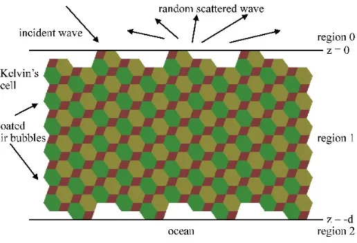
Waves and foam are two primary features that cause the microwave emission changes relative to calm
sea surface [4]. The foam covered on the ocean surface (see Fig. 1) could be classified into three
types [17]: the whitecap, which is active with short life spans; the white water, which is a form of bubbly and unstable water; and the static foam, which is also named residual foam as it is generated after the decaying of whitecaps. In general, the whitecaps are treated, particularly, for their dynamic and time-varied shapes.
When bubbles aggregate together, they are forced into polyhedral shapes as the gravity extracts most of the liquids from their interstices. The bubbles on the top level of the foam layer are polyhedral with lower water fractions, whereas the bubbles on the bottom of the foam layer tend to be small with higher water fractions and almost buried in seawater [5, 6, 9]. Fig. 2 shows the vertical structure of the foam layer and the geometric shape of the bubbles.
Figure 1. Foam layer covered on ocean surface (Photograph from Eastern China Sea, Wind Scale 8, December 2015).
Figure 2. Vertical structure of foam layer.
(a) single Kelvin cell (b) discretization of seawater film
Figure 3. Geometry of Kelvin’s Tetrakaidecahedron structure.
The foam has least surface area to maintain the bubbles stable that forces the bubbles into polyhedral shapes [12]. The surface of Kelvin’s structure consists of six squares and eight hexagons, with a minimal seawater film thickness on each face. These bubbles aggregate through the body-centered-cubic (BCC) structure for constructing the foam layer [12].
Note that the size of air bubbles is randomly distributed owing to the dynamic changing processes in the foam layer. The statistical distribution may be achieved through the randomness of the thickness
t of the seawater film, which is determined by the water fraction (the water content in a provided
volume) fw in the foam layer. For a Kelvin’s Tetrakaidecahedron structure with a side-length ℓ, the
relationship between the thickness tand the water fraction fw is expressed as [13]
fw = ∫
dt(6 + 12
√
3)t
8√2ℓ p(t) =
(6 + 12√3)⟨t⟩
8√2ℓ (1)
3. SCATTERING AND EMISSION MODELING APPROACHES 3.1. Foam Layer Scattering: Method of Moments Formulation
Figure 4. Geometrical configuration for thermal emission from a foam-covered ocean surface.
Considering a vector plane waveEinc(⃗r) impinging upon a foam layer embedded in air, as shown in
Fig. 4, by noting the relative permittivity of seawater film being without coordinate dependence, then the VIE is
E(⃗r) =Einc(r⃗) +k20(εr−1) ∫
G(⃗r, ⃗r′)·E(⃗r′)d⃗r′ (2)
where k0 is the wave number in air, εr the relative permittivity of the seawater film, and G(⃗r, ⃗r′) the
dyadic Green’s function in free space:
G(⃗r, ⃗r′) = (
I+∇∇
k02
)
eik0|⃗r−⃗r′|
4π|⃗r−⃗r′| (3)
In the above equation, ¯r stands for the coordinate of observation point, and ¯r′ corresponds to
the coordinate of source point. The VIE can be discretized by DDA through digitizing Kelvin’s
Tetrakaidecahedron structure’s seawater film intoN segments
Em(⃗r) =k02(εr−1) N ∑
n=1
n̸=m
G(⃗r, ⃗r′)·En(⃗r′)∆Vn+Eminc(⃗r) +Eselfm (⃗r) m, n= 1,2,· · · , N (4)
where ∆Vn is the volume of the nth segment, and the self-term can be expressed by using dyadic L
operator, as
Eselfm (⃗r) =k02(εr−1) (
– ∫Vmd⃗r
′G(⃗r
m, ⃗r′)−
L
k2 0
)
·Em (5)
where –∫ denotes a principle value of the integral, which can be computed by numerical integration; the
operatorL is determined by the shapes of least segments in DDA, for example, a sphere or cube with
L=I/3 [19]. As the least segments of the seawater film are nonspherical or cubic, we use theLoperator
for general cases derived by electrostatics theory [20], expressed as
L= ∫
Sδ
dS′ Rˆ ′nˆ′
4π|r¯−r¯′| (6)
The DDA equation can now be transformed into a matrix equation with dimensions of 3N ×3N
by using the method of moments (MOM) with point matching:
[Zxx] [Zxy] [Zxz]
[Zyx] [Zyy] [Zyz]
[Zzx] [Zzy] [Zzz]
EExy
Ez =
Eincx Eincy Eincz
(7)
The elements in the impedance matrix are evaluated by
Zij,mn= {
−k20(εr−1)∆VnGij(⃗rm, ⃗rn),
I−k02(εr−1)Zselfij,mm,
∀m̸=n
∀m=n i, j =x, y, z; m, n= 1, 2, · · ·, N (8)
where the diagonal terms for each sub-matrix are expressed as
Zselfij,mm = ∫
∆Vm−Vδ
Gij(⃗rm, ⃗r′)d⃗r′−
L
k02 (9)
For the matrix equation (7), the 3D volume UV fast algorithm [13] is applied, and the computation
complexity and memory requirement are reduced toO(3Nlog 3N).
3.2. Absorption, Scattering and Extinction Coefficients of Foam Layer
Once the matrix equation (7) is solved, the power absorbed by the foam layer can be calculated by
Pabs =
1 2ω N ∑ n=1 ∫
∆Vn
d⃗rε′′r(⃗r)|En(⃗r)|2 (10)
and the absorption coefficients κa is readily computed by
κa=
Pabs 1 2η0 |E
inc|2V =
ωε”rη0
|Einc|2V
N ∑
n=1
|En(⃗r)|2∆Vn (11)
where V is the total volume of the foam layer, ω the angular frequency of the incident wave, ε′′r the
imaginary part of permittivity of the seawater film, andη0 the free-space wave impedance.
Now, the total scattered powerPs, in far field, can be computed by
Ps=
1
2η0
∫ 2π
0
dϕs
∫ π
0
dθssinθs(Esv2 +Esh2 ) (12)
where the Esv and Esh are the vertical and horizontal polarized scattered fields, respectively. The
incoherent scattered powerPsnc is expressed as
Psnc= 1
2η0
∫ 2π
0
dϕs
∫ π
0
dθssinθs× {⟨
|Esv− ⟨Esv⟩|2
⟩ +
⟨
|Esh− ⟨Esh⟩|2
⟩}
(13)
where the angle bracket denotes the ensemble average over realizations.
It follows that the scattering coefficientsκs is computed using the following expression:
κs=
Psnc
1
2η|Einc(⃗r)|
2
V (14)
Finally, the extinction coefficientκe is the sum of absorption coefficient and scattering coefficient:
Sea water Foam water
Air ut
ul
uu
ud
τ=0
τ=τ0
θ
zˆ
Figure 5. Geometry of emission from foam-covered ocean surface layer.
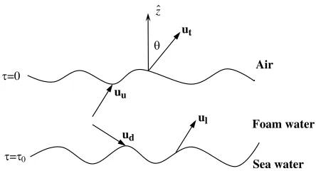
3.3. Emission from Foam-covered Ocean Surface: Matrix Doubling Method
The geometry of the emission model for a foam-covered ocean surface is shown in Fig. 5. Within the
foam layer, contributions to the total emission utfrom the foam-covered ocean surface can be categorized
into three types of sources: the up-welling sourceuu, the down-welling sourceud in the foam layer, and
the emission from seawaterul.
Owing to the presence of volume scattering and volume-interface interactions in the foam layer, the three emission sources undergo multiple scattering processes. The total emission from the foam-covered ocean surface can be written as
ut=Luuu+Ldud+Llul (16)
where Lu,Ld, andLl are the multiple scattering operators, and the emission components ul from the
lower ocean half-space can be determined by using Rayleigh-Jean’s law directly with its emissivity el
as [15]
ul =el(KT /λ2)[µε/µ0ε0] (17)
where K is the Boltzmann constant; T is the seawater physical temperature in Kelvin; λ is the
wavelength;µand εare the permeability and permittivity of seawater, respectively.
In the matrix doubling method [15, 16], the forward and backward single scattering matrices of the foam layer, and the reflection and transmission matrices of the air-foam and foam-seawater interfaces can be obtained for both incident and reversed incident directions. By combining the scattering matrices of the foam layer and the effective reflection and transmission matrices of the interfaces, the multiple
operatorLu of the up-welling effective emission sourceuu is expressed as follows:
Lu = Q˜af+Q˜afTt∗R˜fwTtR˜fa+Q˜afT∗tR˜fwTtR˜faTt∗R˜fwT∗tR˜fa+· · ·
= Q˜af(I−T∗tR˜fwTtR˜fa)−1 (18)
For the down-welling effective emission source ud, the multiple scattering operator Ld is expressed as
Ld = Q˜afTt∗R˜fw+Q˜afT∗tR˜fwTtR˜faT∗tR˜fw+· · ·
= Q˜af(I−T∗tR˜fwTtR˜fa)T∗tR˜fw (19)
and for the seawater effective emission source ul
Ll = Qaf˜ T∗t+Qaf˜ T∗tRfwTt˜ RfaT˜ ∗t +QafT˜ ∗tRfwTt˜ RfaT˜ t∗RfwTt˜ RfaT˜ ∗t+· · ·
= Qaf˜ (I−T∗tRfwTt˜ Rfa˜ )−1T∗t (20)
where St, Tt, S∗t, and T∗t are the scattering matrices of the foam layer; R˜af, Q˜fa, R˜fa, and Q˜af are
the effective reflection and transmission matrices of the air-foam interface, whereas Rwf˜ , Qfw˜ , Rfw˜ ,
and Qwf˜ are the effective reflection and transmission matrices of the foam-seawater interface for both
incident and reversed incident directions.
The azimuthal angle dependence may be eliminated using the Fourier series expansion and harmonic
factor of the corresponding items, we can write the multiple scattering operators of up-welling, down-welling, and seawater effective emission sources as [15]
Lu = f02Q˜0af(I−f02Tt0∗R˜0fwT0tR˜0fa)−1 (21)
Ld = f02Q˜0af(I−f02T0t∗R˜0fwT0tR˜0fa)T0t∗R˜0fw (22)
Ll = f02Q˜0af(I−f02T0t∗R˜0fwT0tR˜0fa)− 1
T0t∗ (23)
where f0 = 0.5 and the subscript “0” stands for the zeroth Fourier component in the Fourier series of
these matrices.
Finally, for a foam layer with a thicknessτ0, the harmonic expressions of the up-welling and
down-welling effective emission sources in the foam layer, which are related to the scattering matrices of the
foam layer and its physical temperature profile T(τ), can be obtained by integrating over the thickness
of the foam layer [15]
uu(τ0) =
∫ τ0
0
dτT0t∗(τ)[I−f02St0(τ0−τ)S0t∗(τ)]−1
×[I+S0t(τ0−τ)](1−a)
K λ2εeM−
1T(τ) (24)
ud(τ0) =
∫ τ0
0
dτT0t∗(τ0−τ)[I+S0t∗(τ)](1−a)
×[I−f02S0t∗(τ)S0t(τ0−τ)]−1
K λ2εeM−
1T(τ) (25)
whereais the single albedo,εe the effective permittivity of the foam layer, and Mthe diagonal matrix
of the directional cosine.
3.4. Surface Scattering and Phase Matrix
The bistatic scattering coefficients γ(θs, ϕs;θi) (different from previous scattering coefficients κs) of
ocean surface can be determined using the IEM model [14, 22]. Then, the surface scattering phase matrix is expressed as
P(θs, ϕs;θi) =
γ(θs, ϕs;θi)
4πcosθi
(26)
and the emissivity of the ocean half-space with a rough surface boundary is calculated by
ep(θi) = 1−Rpexp[−(khcosθi)2]−
∫ 2π
0
∫ π/2
0
γp(θs, ϕs;θi)
4πcosθi
sinθsdθsdϕs, p=h, v (27)
where h is the root-mean-square (RMS) height of the rough ocean surface, Rp the Fresnel reflection
coefficient forp-polarization, andγp =γhp+γvp.
As the bubbles in the foam layer are densely packed, neither the far field nor the point size scatterer assumption is valid for this case. As a result, the near field and size effects of the bubbles should be considered. Furthermore, the volume scattering of the foam layer is relatively weak compared to its absorption; hence, fully coherent interactions and multiple scattering effects within the foam layer should be considered for higher accuracy. As the size of the bubbles relative to wavelength is small [6] and
satisfies the Rayleigh approximation condition (kr ≪ 1), the Rayleigh phase matrix [23] that includes
range and size-dependent terms in the scattered field is utilized in this study.
Another key parameter is the effective permittivity of the foam layer, which in turn determines the Fresnel reflection coefficients of air-foam and foam-seawater interfaces in the IEM surface scattering model. The quadratic mixing formula [24] is used for calculating the effective permittivity [10]
√
εe= (1−fw) +fw√εr (28)
4. PARAMETERS FOR MODEL ANALYSES
The key model parameters are as follows:
T Physical temperature of the seawater and the foam layer;
S Seawater salinity;
f The operating frequency;
εr Seawater (also the seawater film) permittivity;
τ0 Thickness of the foam layer;
fw Water fraction in the foam layer;
Nc Number of Kelvin’s cells;
ℓSide-length of Kelvin’s cells;
V Total volume of the foam layer;
tj Thickness of thejth cell wall;
⟨t⟩ Ensemble average thickness of the seawater film;
p(t) Probability density function of the cell-wall thickness;
Frequencies at 1.5 GHz (L-band), 5.0 GHz (C-band), 10.8 GHz (X-band), 18.0 GHz (Ku-band), and 36.5 GHz (Ka-band) were selected. As the permittivity for either the seawater or the seawater film is a function of frequency, sea surface temperature, and seawater salinity, we utilize the Debye seawater
permittivity model [25] by setting the seawater temperature and salinity at 283 K and 35‰as provided
in [5]. The permittivities of seawater at five frequencies are listed in Table 1.
Table 1. Permittivity as a function of frequency.
Frequency (GHz) 1.5 5.0 10.8 18.0 36.5
Permittivityεr 74.714+i53.705 66.499+i37.428 49.149+i40.105 29.090+i37.362 13.448+i24.784
As reported in [6], the bubble radius in the natural sea foam layer is a random variable and can be described using the Gamma distribution with a mean value of 0.781 mm, and the most probable
radius was observed to be 0.595 mm. It follows that the side-length ℓ of Kelvin’s structure was set to
0.448 mm. The equivalent radius of a Kelvin’s structure was approximately 0.663 mm, which is close to
the mean value or probable radius of the natural sea foam bubbles. A total of Nc = 512 (8×8×8)
cells were aggregated together through the BCC structure to form a foam layer with a fixed thickness
of approximately 1 cm. Note that the total volume can be calculated by V = 8√2ℓ3Nc. The number
of unknowns in (7) is determined by the number of Kelvin’s cells Ncand the discretization factorn0 of
a Kelvin’s cell. The discretization factor n0 determines the number of least segments on each surface
of each Kelvin’s structure. For a givenn0, the square face of Kelvin’s cell acquired n20 least segments,
whereas for a hexagon face, the number of least segments turns out to be 3n20. For example, in Fig. 3(b),
the discretization factor n0 = 5. However, in the BCC structure, Kelvin’s structure shares half of its
faces with the adjacent Kelvin’s cells. Thus, for one Kelvin’s cell, the number of least segments is
3×n20+ 4×3n20 = 15n20. Then, the total unknowns is
N = 3×Nc×15n20 (29)
In this study, the discretization factor is set at n0 = 2, and the side-length of the least segment is
0.224 mm, which yields 10 sample points per wavelength in seawater at the highest operating frequency (36.5 GHz) and provides sufficient computation accuracy. The total number of unknowns is calculated
by (29) asN = 92160. We used 10 realizations for each case. For each realization, it took about 10–30
minutes to complete the simulation on a single 2.3-GHz CPU, with a memory of 16 GB.
Table 2. Numerical simulation parameters.
Parameter T (K) S (‰) τ0 (cm) Nc ℓ(mm) V (cm3) fw (%) N
Value 283 35 1.0 512 0.448 0.521 0.5–10.5 92160
It is commonly accepted that the probability density function of the average thickness of seawater
film,p(t), follows the Rayleigh distribution [12]
p(t) = t
σ2 exp
(
− t2
2σ2
)
(30)
where σ = √2/π⟨t⟩. Once the water fraction in the foam layer is known, the mean thickness of the
seawater film can be computed.
5. SCATTERING AND ABSORPTION COEFFICIENTS OF FOAM LAYER
This section presents the angular and frequency dependence of V- and H-polarized absorption and
scattering coefficients.
5.1. Absorption Coefficients of Foam Layer
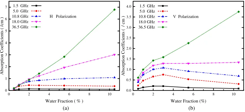
Figure 6 shows theH- andV-polarized absorption coefficients (Np/cm) as a function of water fraction
at an incident angle of 30◦. It can be observed that the absorption coefficients at higher frequencies are
larger than those at lower frequencies for both polarizations.
(a) (b)
0 2 4 6 8 10
0 1 2 3 4 5 6 7
Absorption Coefficients
( /cm )
Water Fraction ( % )
1.5 GHz 5.0 GHz
10.8 GHz H Polarization 18.0 GHz
36.5 GHz
0 2 4 6 8 10
0.0 0.5 1.0 1.5 2.0 2.5 3.0 3.5 4.0
Absorpti
on Coefficients ( / cm )
Water Fraction (%)
1.5 GHz 5.0 GHz
10.8 GHz V Polarization 18.0 GHz
36.5 GHz
Figure 6. Absorption coefficient as a function of water fraction at different frequencies with an incident
angle of 30◦. (a) For horizontal polarization; (b) for vertical polarization.
For H-polarization, the absorption coefficient initially increases with water fraction and quickly
saturates for frequencies from 1.5 to 10.8 GHz, whereas, it monotonically increases with water fraction
for frequencies greater than 18 GHz. For theV-polarized absorption coefficient, its dependence on water
fraction is more complicated, as illustrated in Fig. 6(b). The frequency behavior of the V-polarized
It is known that the skin depth at low frequencies is larger than that at high frequencies in the pure seawater. In addition, as reported in [26], the skin depth in the foam layer is larger than that in pure seawater. Considering these, the plots in Fig. 6 can be physically explained as follows. For frequency at 36.5 GHz, with the least skin depth in pure seawater among these operating frequencies, the absorption coefficient increases with the increase of water fraction, which corresponds to a steepest decreasing of its skin depth in the foam layer, because the pure seawater effect is applied with increasing water fraction. At lower frequencies, particularly the L-band, and thus larger skin depth, the wave penetrates deeper into the foam layer. Hence, the absorption coefficients at these lower frequencies are prone to saturate with increasing water fraction in the foam layer. In other words, the impact of skin depth with water fractions are implicitly illustrated in Fig. 6 for all frequencies, in a way that the absorption coefficient exhibits different sensitivities to water fractions in the foam layer.
Figure 7 shows a comparison of absorption coefficients between H- and V-polarizations at three
operating frequencies with an incident angle of 30◦. At smaller water fractions, the V-polarized
absorption coefficients are larger than the H-polarized ones. However, as the water fraction increases,
theV-polarized absorption coefficients saturate and then decrease quicker than theH-polarized cases;
eventually, theV-polarized absorption coefficients reduce below theH-polarized ones. From Fig. 7, it
is also observed that the polarization dependence of absorption coefficients at 18 GHz is significantly different for water fraction greater than 3%.
0 2 4 6 8 10
0.0 0.5 1.0 1.5 2.0 2.5 3.0
Ab
so
rp
ti
on Co
efficients
( /cm
)
Water Fraction ( % )
Frequency V H 5.0 GHz 10.8 GHz 18.0 GHz
Figure 7. Comparison of absorption coefficients between H- andV-polarizations at an incident angle
of 30◦.
The angular dependence of absorption coefficients for both polarizations at 18.0 GHz, as shown in
Fig. 8, shows that theH-polarized absorption coefficient is considerably less dependent on the incidence
angle than that for theV-polarized one, regardless of the water fraction. Higher water fraction resulting
in larger absorption is again observed from the figure. The plots of absorption coefficients versus incident
angles for several frequencies at 5.5% water fractions are shown in Fig. 9. For V-polarization, the
absorption decreases at larger incidence angles, whereas for H-polarization it remains almost
angle-independent for all frequencies under consideration.
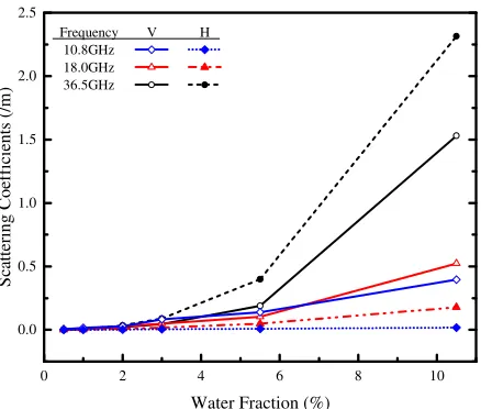
5.2. Scattering Coefficients of Foam Layer
TheH- andV-polarized scattering coefficients (Np/m) at 10.8, 18, and 36.5 GHz with 30◦incident angle
are plotted in Fig. 10. The volume scattering coefficients of foam layer are negligible at low frequencies. As shown in Fig. 10, the volume scattering coefficient of foam layer increases with increasing water fraction at all selected frequencies, and its polarization dependence is negligible at water fractions less
than 2%. At 10.8 and 18 GHz, the H-polarized scattering coefficient is smaller than the V-polarized
one for larger water fraction; the opposite occurs at 36.5 GHz, at which the V-polarized scattering is
30 35 40 45 50 55 60 0.0
0.5 1.0 1.5 2.0 2.5 3.0
Ab
so
rp
tio
n Co
efficients ( /cm )
Incident Angle ( deg ) Frequency 18.0 GHz
Water Fraction (%) 0.5 2.0 5.5 10.5 V H
Figure 8. Angular dependence of H- and V-polarized absorption coefficients at 18.0 GHz.
30 35 40 45 50 55 60
0.0 0.5 1.0 1.5 2.0
Ab
so
rpti
on Co
efficients
( /cm )
Incident Angle (deg)
Water Fraction 5.5% Frequency V H 1.5 GHz 5.0 GHz 10.8GHz 18.0GHz
Figure 9. Angular dependence of absorption coefficients forH- andV-polarizations at a water fraction of 5.5%.
It is evident from Fig. 10 that, at low water fractions, the foam layer is weakly scattering. Therefore, at low water fraction, it is reasonable to ignore the scattering effects of the foam layer in the incoherent scattering model [11].
6. MODEL ANALYSES OF EMISSION FROM FOAM-COVERED OCEAN SURFACE
This section presents the modeling and analysis of emission from the foam-covered ocean surface. The emission dependence on water fraction at selected frequency and polarizations are provided, along with analyzing the effective emission sources contributing to the total emission.
6.1. Effects of Water Fraction on Emissivity at Different Frequencies and Polarizations
0 2 4 6 8 10 0.0
0.5 1.0 1.5 2.0 2.5
Sc
atterin
g Coefficients
(/m
)
Water Fraction (%) Frequency V H
10.8GHz 18.0GHz 36.5GHz
Figure 10. Scattering coefficients at an incident angle of 30◦ as a function of water fraction forH- and
V-polarizations at different frequencies.
30 35 40 45 50 55 60
0.1 0.2 0.3 0.4 0.5 0.6 0.7
Emissiv
it
y
View Angle ( deg ) Frequency 1.5 GHz
Water Fraction V H 1.0 % 3.0 % 5.5 % Seawater
Figure 11. Emissivity at 1.5 GHz with varied water fractions as a function of view angles.
at relative low water fractions (from 1.0% to 3.0%), and then decreases with increasing water fraction. Fig. 12 shows the emissivity versus incident angles, at 3% water fraction, for 1.5, 10.8, and 36.5 GHz. Note that the emissivity increases monotonically with increasing operating frequencies from 1.5 to 36.5 GHz at 3% water fraction.
For general cases, the water fraction and frequency dependencies of emissivity for both V- and
H-polarizations at a view angle of 45◦ are shown in Fig. 13. For both polarizations and at all selected
operating frequencies, the water fraction and frequency dependencies of emissivity show the same general trends as the special cases presented in Figs. 11 and 12. Although emissivities at all selected operating frequencies have similar dependencies with water fraction and frequency, they exhibit different sensitivities to water fractions; emissivities at high operating frequencies exhibit higher sensitivities to water fractions than the lower ones.
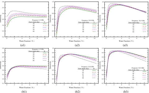
The V- and H-polarized emissivities for view angles from 30◦ to 60◦ at L-, X-, and Ka-bands as
a function of water fraction are illustrated in Fig. 14, where the 0% water fraction implies the planar
pure seawater surface case. It can be observed that the V-polarized emissivity reserves its angular
30 35 40 45 50 55 60 0.4
0.5 0.6 0.7 0.8 0.9 1.0
Emissiv
it
y
View Angle ( deg ) Water Fraction 3.0 %
Frequency V H
1.5 GHz
10.8 GHz
36.5 GHz
Figure 12. Emissivity at 3.0% water fraction with varied operating frequencies as a function of view angles.
(a) (b)
0 2 4 6 8 10
0.3 0.4 0.5 0.6 0.7 0.8 0.9 1.0
Emissivity
Water Fraction ( % ) View Angle : 45°
Frequency ( GHz ) 1.5 5.0 10.8 18.0 36.5
V Polarization
0 2 4 6 8 10
0.3 0.4 0.5 0.6 0.7 0.8 0.9 1.0
Emissivity
Water Fraction ( % ) View Angle : 45° Frequency ( GHz ) 1.5 5.0 10.8 18.0 36.5
H Polarization
Figure 13. Emissivity at all operating frequencies as a function of water fraction. (a) For V
-polarization; (b) forH-polarization.
WhenV-polarized emissivity loses its angular dependence, it explains that the Brewster angle effect
on the planar ocean surface diminishes owing to the existence of a foam layer. Besides, at each operating
frequency, the difference of emissivity between the view angles of 30◦ and 60◦ for the foam-covered case
is smaller than that for the pure seawater surface case, which also explains the vanishing Brewster angle
effects. Similarly, the difference of theH-polarized emissivity between the two angles reflects the descent
speed of emissivity. Thus, the existence of the foam layer reduces the descent speed of theH-polarized
emissivity at low water fractions, and the descent speed increases again at high water fractions (which is approximately 10.5%), as shown in Fig. 11.
6.2. Emission Polarization Index of Foam-Covered Ocean Surface
(a1) (a2) (a3)
(b1) (b2) (b3)
0 2 4 6 8 10
0.2 0.3 0.4 0.5 0.6 0.7 0.8 Em is si vi ty
Water Fraction ( % )
Frequency 1.5 GHz View Angle (deg) V
30
40
45
50
60
0 2 4 6 8 10 0.4 0.5 0.6 0.7 0.8 0.9 1.0 Emi ssi vit y Water Fraction ( % ) Frequency 10.8 GHz View Angle (deg) V 30
40
45
50
60
0 2 4 6 8 10 0.4 0.5 0.6 0.7 0.8 0.9 1.0 Em issi vi ty Water Fraction ( % ) Frequency 36.5 GHz View Angle (deg) V 30
40
45
50
60
0 2 4 6 8 10 0.1 0.2 0.3 0.4 0.5 0.6 0.7 0.8 0.9 Em is si vi ty Water Fraction ( % ) Frequency 1.5 GHz View Angle (deg) H 30
40
45
50
60
0 2 4 6 8 10 0.2 0.3 0.4 0.5 0.6 0.7 0.8 0.9 1.0 Em is si vi ty Water Fraction ( % ) Frequency 10.8 GHz View Angle (deg) H 30
40
45
50
60
0 2 4 6 8 10 0.2 0.3 0.4 0.5 0.6 0.7 0.8 0.9 1.0 Em is si vi ty Water Fraction ( % ) Frequency 36.5 GHz View Angle (deg) H 30
40
45
50
60
Figure 14. Emissivity at sample view angles from 30◦ to 60◦ as a function of water fraction. (a)
For V-polarization; (b) For H-polarization. Columns (1), (2), and (3) are, respectively, at L-, X-, and
Ka-bands.
subsection. The polarization index is defined as
P I= ev−eh
ev+eh
(31)
Similar to the angular dependence and polarization effects of emissivity presented in the preceding
subsections, the polarization indexes at L-, X-, and Ka-bands at sampling view angles from 30◦ to 60◦
are plotted as a function of water fraction in Fig. 15. It is observed that with increasing water fraction, the polarization indices initially decrease and then saturate at low frequencies and increase subsequently at higher frequencies.
As depicted in Fig. 15, the polarization loses its angular dependence at approximately 3.0% water fraction at high operating frequencies, whereas the angular dependence reserves at low operating frequencies such as the L-band. In particular, a strongest depolarization at the Ka-band occurs at
a low water fraction as it is closer to zero. In Fig. 16, the polarization indices at a view angle of 45◦ for
the foam-covered case are also plotted as a function of water fraction at all operating frequencies. It can be observed that, the polarization index decreases monotonically with increasing frequency at all water fractions, and exhibits different sensitivities to water fractions at each operating frequency.
6.3. Emission from Effective Emission Source
Sources for the total emission from the foam-covered ocean surface can be categorized into three types: up-welling, down-welling, and contribution from seawater. In this subsection, the emission from these three effective emission sources is discussed for exploring the mechanism of emission from the
foam-covered ocean surface. Without loss of generality, the emission from up-welling effective source Luuu,
down-welling effective sourceLdud, and seawater emissionLlul at L- and Ka-bands at a view angle of
(a) (b) (c)
0 2 4 6 8 10
0.0 0.1 0.2 0.3 0.4 0.5 Po larization Inde x
Water Fraction ( % ) Frequency 1.5 GHz View Angle (deg) Index
30
40
45
50
60
0 2 4 6 8 10 0.0 0.1 0.2 0.3 0.4 0.5 Po larization Inde x Water Fraction ( % ) Frequency 10.8 GHz View Angle (deg) Index 30
40
45
50
60
0 2 4 6 8 10 0.0 0.1 0.2 0.3 0.4 0.5 Po lari za ti on Ind ex Water Fraction ( % ) Frequency 36.5 GHz View Angle (deg) Index 30
40
45
50
60
Figure 15. Polarization index at sample view angles from 30◦ to 60◦ as a function of water fraction: (a) at L-band; (b) at X-band; (c) at Ka-band.
0 1 2 3 4 5 6 7 8 9 10 11
0.00 0.02 0.04 0.06 0.08 0.10 0.12 0.14 0.16 0.18 Polarization I nde x
Water Fraction (%)
View Angle 45° Frequency (GHz) PI 1.5 5.0 10.8 18.0 36.5
Figure 16. Polarization index at a view angle of 45◦ as a function of water fraction for all operating frequencies.
For the L-band, because of the large skin depth and low sensitivity to water fractions in the foam layer, the seawater emission dominates the total emission. As the effective permittivity gradually approaches to that of pure seawater with increasing water fraction, the foam-seawater interface effects tend to be vanished. Hence, the emission from seawater increases with the increase of water fraction and the polarized emissivity difference of the seawater at the L-band decreases, and tends to be stable
eventually. As an inverse process of the up-welling emission, theH-polarized emission from the
down-welling emission source is larger than that ofV-polarized owing to the reflection from the foam-seawater
interface. Once the effects of the foam-seawater interface gradually recedes with increasing water
(a) (b)
0 1 2 3 4 5 6 7 8 9 10 11
0.00 0.05 0.10 0.15 0.20 0.25 0.30 0.35 0.40 0.45
Em
issivity
Water Fraction (%)
Frequency 1.5 GHz Emission Source V H Up-welling
Down-welling Seawater
0 1 2 3 4 5 6 7 8 9 10 11
0.0 0.1 0.2 0.3 0.4 0.5 0.6 0.7 0.8 0.9
Em
issivit
y
Water Fraction (%)
Frequency 36.5 GHz Emission Source V H Up-welling Down-welling Seawater
Figure 17. The emissivity from three emission sources: (a) at L-band; (b) at Ka-band.
water fraction, and both emissions from the down-welling source and the seawater decrease rapidly with increasing water fraction. It is of interest to note that the polarization difference of emissivity, which monotonically increases with the increase of water fraction, is more pronounced at the Ka-band than that at the L-band. It can be deduced that for the Ka-band, the emission is strongly dependent on the foam layer and the air-foam interface. In summary, the important characteristics of these three effective emission sources are expressed as follows:
(1) The seawater emission is the dominant source for total emission at lower frequency. Moreover, it may become stronger due to the variations of water fraction in the foam layer. This is also explained by a larger polarization index at a lower frequency.
(2) The emission from a down-welling effective emission source is sensitive to the water fraction in the foam layer since it is mainly due to the reflection from the foam-seawater interface. This could explain the tendency of polarization index as a function of water fraction in Figs. 15 and 16 at different operating frequencies. The down-welling emission exhibits a higher H-polarization than V-polarization. (3) The up-welling emission mainly emerges from the foam layer and the effects of the air-foam interface. The latter almost has no bearing on the emission from the up-welling emission source at low water fractions; for a certain water fraction, the effects of air-foam interface are more obvious at high frequencies. Thus, the strongest depolarization at the Ka-band originates the prominent contributions of total emission from the foam layer, and then the polarization index increases with the increase of water fraction.
7. CONCLUSIONS
on frequency. The seawater emission is the dominant source for total emission at lower frequency. The emission from the down-welling effective emission source is sensitive to the water fraction in the foam layer because it is mainly due to the reflection from the foam-seawater interface. The down-welling
emission exhibits a higherH-polarization thanV-polarization. The up-welling emission mainly emerges
from the foam layer and the effects of the air-foam interface. As far as water fraction is concerned, the polarization indexes decrease at first and saturate at low frequencies and increase subsequently at higher frequencies when the water fraction increases.
Although the water fraction profile has been applied continuously, the interface effects of each level in the foam layer should be considered, particularly, for the dominant effects of the boundary between the static foam layer and the white water at low operating frequencies, as the water fraction varies from 0% to 100% in the incoherent model and both the patterns of foam are included.
Some issues for further studies are noted to conclude the paper. The bubble shapes in the static foam layer (polyhedral) and the white water (spherical) are different and the boundary of water fraction between static foam and white water should be exploited. Particularly, a comprehensive investigation on the roughness effects of the ocean surface on the emissivity should be conducted. The emission from a foam layer with multilevel structure should be investigated and compared with the experimental measurements.
ACKNOWLEDGMENT
This work was supported in part by the National Science Foundation of China under Grant 41171291 and 41531175 and in part by the RADI Director. The author thanks Dr. Yu Liu, Dr. JiangyuanZeng, Dr. Ming Jin, Miss Ying Yang, and Mr. Chong Peng for their selfless help and valuable suggestions.
APPENDIX A. FORMULATION OF L OPERATOERS FOR LEAST SEGEMENTS
In this study, two types of least segment are considered in the discretization of square and diamond surfaces on Kelvin’s structure: One is the parallelepiped with quadrate upper and lower surfaces (least segments on square surfaces in Fig. 3(b)), and the other is a parallelepiped with diamond upper and lower surfaces (least segments on diamond surface in Fig. 3(b)). For the field in the source region of
these least segments, we notice the properties of L operator in [19].
First, theL operator is a diagonal matrix
L=
[ L
xx 0 0
0 Lyy 0
0 0 Lzz
]
(A1)
and its diagonal elements obey
T race(L) =Lxx+Lyy+Lzz = 1 (A2)
If the least segments with geometrical symmetry are directional, for example, in the x-y plane, then we
have
Lxx=Lyy= (1−Lzz)/2 (A3)
The direction of the thickness of the seawater film is defined in thez-axis. For the first type least
segments with quadrate upper and lower surfaces with geometrical symmetry in the x-y plane, the L
operator for the z direction can be derived by combining the properties of the L operator and the
integral identities [27] as
Lzz =
2
πtan
−1 ab
c(a2+b2+c2)1/2 (A4)
where a=bin this case, which represents the side-length of the parallelepiped in the x-y plane and c
is the thickness of the seawater film. Then the components of the Loperator in the xand y directions
can be calculated by using (A3).
(x,y,z) system to (u,v,w) system as suggested in [28]. Thus, in the new (u,v,w) coordinate system,
only the components of theLoperator in thewdirection should be calculated as it is symmetric in the
u-v plane similar to the first type least segments. The w components of theL operator for the second
least segments are derived by
Lww= √
3
π
∫ δu
2
−δu
2
du (u+δv)δw
(3u2+δ2
w) √
4u2+2δ
vu+δv2+δw2
(A5)
where δu, δv, and δw denote the side-lengths of the least segments in the (u, v, w) coordinate system,
and (A5) is then calculated through numerical integration methods. Similarly, the components in the
u and v directions can be obtained by using (A3).
REFERENCES
1. Bettenhausen, M. H., C. K. Smith, R. M. Bevilacqua, N. Y. Wang, P. W. Gaiser, and S. Cox,
“A nonlinear optimization algorithm for WindSat wind vector retrievals,” IEEE Trans. Geosci.
Remote Sens., Vol. 44, No. 3, 597–610, 2006.
2. Andreas, E. L., “Spray-mediated enthalpy flux to the atmosphere and salt flux to the ocean in the
high winds,”J. Phys. Oceanogr., Vol. 40, No. 3, 608–619, 2010.
3. Smith, P. M., “The emissivity of sea foam at 19 and 37 GHz,”IEEE Trans. Geosci. Remote Sens.,
Vol. 26, No. 5, 541–547, 1988.
4. Stogryn, “The emissivity of sea foam at microwave frequencies,” J. Geophys. Res., Vol. 77, No. 9,
169–171, 1972.
5. Rose, L. A., W. E. Asher, S. C. Resing, P. W. Gaiser, D. J. Dowgiallo, K. A. Horgan, G. Farquharson, and E. J. Knapp, “Radiometric measurements of microwave emissivity of foam,” IEEE Trans. Geosci. Remote Sens., Vol. 40, No. 12, 2619–2625, 2002.
6. Camps, A., M. Vall-llosera, R. Villarino, N. Reul, B. Chapron, I. Corbella, N. Duffo, F. Torres, J. J. Miranda, R. Sabia, A. Monerris, and R. Rodriguez, “The emissivity of foam-covered water
surface at L-Band: Theoretical modeling and experimental results from the Frog 2003 field
experiment,” IEEE Trans. Geosci. Remote Sens., Vol. 43, No. 5, 925–937, 2005.
7. Chen, D., L. Tsang, L. Zhou, S. C. Reising, W. E. Asher, L. A. Rose, K. H. Ding, and C. T. Chen “Microwave emission and scattering of foam based on Monte Carlo simulations of dense media,” IEEE Trans. Geosci. Remote Sens., Vol. 41, No. 4, 782–790, 2003.
8. Raizer, V., “Macroscopic foam-spray models for ocean microwave radiometry,”IEEE Trans. Geosci.
Remote Sens., Vol. 45, No. 10, 3138–3144, 2007.
9. Anguelova, M. D., “Complex dielectric constant of sea foam at microwave frequencies,”J.Geophys.
Res.: Oceans, Vol. 112, No. C8, 2008.
10. Anguelova, M. D. and P. M. Gaiser, “Microwave emissivity of sea foam layers with vertically
inhomogeneous dielectric properties,”Remote Sens. Environ., Vol. 139, No. 12, 81–96, 2013.
11. Yueh, S. H., “Modeling of wind direction signals in polarimetric sea surface brightness
temperatures,”IEEE Trans. Geosci. Remote Sens., Vol. 35, No. 6, 1400–1418, 1997.
12. Weaire, D. and S. Hutzler, The Physics of Foam, Clarendon Press, Oxford, 1999.
13. Xu, P., L. Tsang, and D. Chen, “Application of the multilevel UV method to calculate microwave
absorption and emission of the ocean foam with Kelvin’s Tetrakaidecahedron structure,” Microw.
Opt. Technol. Lett., Vol. 45, No. 5, 445–450, 2005.
14. Fung, A. K., Z. Li, and K. S. Chen, “Backscattering from a randomly rough dielectric surface,” IEEE Trans. Geosci. Remote Sens., Vol. 30, No. 2, 335–359, Mar. 1992.
15. Fung, A. K., Microwave Scattering and Emission Models and Its Applications, Artech House,
Norwood, Massachusetts, 1994.
16. Tjuatja, S., A. K. Fung, and J. Bredow, “A scattering model for snow-covered sea ice,” IEEE
Trans. Geosci. Remote Sens., Vol. 30, No. 4, 804–810, 1992.
17. Ulaby, F. T., R. K. Moore, and A. K. Fung,Microwave Remote Sensing: Active and Passive, Vol. 3,
18. Reul, N. and B. Chapron, “A model of sea-foam thickness distribution for passive microwave remote
sensing applications,”J. Geophys. Res., Vol. 108, No. C10, 894–895, 2003.
19. Yaghjian, A. D., “Electric dyadic Green’s functions in the source region,” Proc. IEEE, Vol. 68,
No. 2, 248–263, 1980.
20. Tsang, L., J. A. Kong, and K. H. Ding, Scattering of Electromagnetic Waves: Numerical
Simulation, Wiley, New York, 2001.
21. Fung, A. K. and H. J. Eom, “A theory of wave scattering from an inhomogeneous layer with an
irregular interface,” IEEE Trans. Antennas Propag., Vol. 29, No. 6, 899–910, 1981.
22. Fung, A. K. and K. S. Chen,Microwave Scattering and Emission Models for Users, Artech House,
Boston, 2010.
23. Fung, A. K., S. Tjuatja, J. W Bredow, and H. T. Chuah, “Dense medium phase and amplitude
correction theory for spatially and electrically dense media,”Proc. Int. Geosci. Remote Sens. Symp.,
Vol. 2, 1336–1338, 1995.
24. Sihvola, A., Electromagnetic Mixing Formulas and Applications, The Institute of Electrical
Engineers, London, 1999.
25. Klein, L. A. and C. T. Swift, “An improved model for the dielectric constant of sea water at
microwave frequencies,”IEEE Trans. Antennas Propag., Vol. 25, No. 1, 104–111, 1977.
26. Anguelova, M. D. and P. W. Gaiser, “Skin depth at microwave frequencies of sea foam layers with
vertical profile of void fraction,” J. Geophys. Res.: Oceans, Vol. 116, No. C11, 2011.
27. Gradshteyn, I. S. and I. M. Ryzhik,Table of Integrals, Series and Products, 7th Edition, Academic
Press, New York, 2007.
28. Chew, W. C., J. M. Jin, E. Michielssen, and J. M. Song,Fast Efficient Algorithm in Computational