Structured Generative Models of Continuous Features for Word Sense
Induction
Alexandros Komninos Department of Computer Science
University of York York, YO10 5GH
United Kingdom
Suresh Manandhar Department of Computer Science
University of York2 York, YO10 5GH
United Kingdom
Abstract
We propose a structured generative latent variable model that integrates information from mul-tiple contextual representations for Word Sense Induction. Our approach jointly models global lexical, local lexical and dependency syntactic context. Each context type is associated with a latent variable and the three types of variables share a hierarchical structure. We use skip-gram based word and dependency context embeddings to construct all three types of representations, reducing the total number of parameters to be estimated and enabling better generalization. We describe an EM algorithm to efficiently estimate model parameters and use the Integrated Com-plete Likelihood criterion to automatically estimate the number of senses. Our model achieves state-of-the-art results on the SemEval-2010 and SemEval-2013 Word Sense Induction datasets.
1 Introduction
Word Sense Induction (WSI) aims to automatically discover the different senses of polysemous words by unsupervised processing of text corpora. The related task of Word Sense Disambiguation (WSD) seeks to map the senses of word instances in a specific context to a predefined sense inventory. WSI overcomes the problem of having to define sense inventories, which may not have the appropriate granularity for all applications, and the effort of updating them for new domains or novel senses (Klapaftis and Manandhar, 2013). WSI is a challenging task that remains largely unsolved, but has important applications to a large number of tasks that require semantic processing of natural language (Navigli, 2009).
WSI is typically modelled as a clustering task, where the aim is to cluster samples of context represen-tations of ambiguous words. Since context is the only available information to a WSI model, the choice of informative representations is a very important modelling aspect. Broad context related to topic or domain can restrict the possible senses that are applicable to an ambiguous word, but in order to make fine grained distinctions, context on the phrasal or syntactic level is usually needed. Ideally, a WSI sys-tem should incorporate different types of contexts to increase the confidence of its decisions. Combining the information present in different context representations can pose many difficulties in an unsupervised setting. Previous work has combined lexical with syntactic context (Brody and Lapata, 2009; Lau et al., 2012), and topical with local lexical context (Wang et al., 2015).
Another challenge for WSI systems is the need to apply clustering methods in high dimensional spaces of sparse features. Probabilistic latent variable models have been very successful in WSI by inducing latent representations of features that help improve generalization. While the latent variable approach has been very successful for word features, it has not provided considerable advantages when used with syntactic features (Brody and Lapata, 2009; Lau et al., 2012). A possible reason for this is that syntactic features, such as dependency contexts, exhibit much more sparsity than words.
A promising method to overcome the sparsity problem inherent in high dimensional discrete feature spaces is learning a low dimensional representation of the features. Word embeddings are an example of low dimensional vector representations for words learned in an unsupervised manner. The skip-gram
This work is licensed under a Creative Commons Attribution 4.0 International Licence. Licence details: http:// creativecommons.org/licenses/by/4.0/
model (Mikolov et al., 2013) is a very popular technique for learning embeddings that scales to huge corpora and can capture important semantic and syntactic properties of words. Skip-gram embeddings exhibit compositional properties under addition, making them useful for constructing representations of phrases and larger units of text. Recently, the skip-gram model has been extended to learn embeddings of dependency context features (Levy and Goldberg, 2014; Komninos and Manandhar, 2016) that capture additional syntactic information. While word embeddings have been successfully used in many super-vised NLP problems to overcome the problem of sparsity and improve generalization (Turian et al., 2010; Collobert et al., 2011), their application in WSI has been so far very limited.
In this paper, we propose a WSI model to address both the issue of multiple context representations and feature sparsity. Our model is a structured generative model that jointly models topical, phrasal and syntactic context in a hierarchical way. The probabilistic framework allows us to integrate different types of information in a principled way and also allows the application of model selection criteria to automatically determine the optimal number of senses. We address the issue of high dimensional feature spaces when dealing with syntactic features, by using word and dependency feature embeddings. In particular, we use the same skip-gram based model to create representations of all three context types.
We evaluate our model in two competitive benchmarks: SemEval-2010 Task 14: Word Sense Induc-tion and DisambiguaInduc-tion (Manandhar et al., 2010), and SemEval-2013 Task 11: Word Sense InducInduc-tion for graded and non-graded senses (Jurgens and Klapaftis, 2013). The two tasks provide different WSI evaluation frameworks and metrics. The proposed model achieves the state-of-the-art results in both datasets. Code is available athttps://cs.york.ac.uk/nlp/extvec
2 Related Work
Among the most successful WSI systems are probabilistic latent variable models. Brody and Lapata (2009) extend the Latent Dirichlet Allocation (LDA) model (Blei et al., 2003) to combine evidence from different types of contexts. A limitation of this model is that the number of senses needs to be determined manually. Lau et al. (2012) propose using the non-parametric extension of LDA with a hierarchical dirichlet process (Teh et al., 2012) prior (HDP-LDA) to automatically estimate the appropriate number of senses from the data. They showed that HDP-LDA performs significantly better than LDA even when the number of senses is set to the same value. They also experimented with combined syntactic and word features. Syntactic features did not provide any advantage to either of these two LDA type models, but this could be attributed to sparsity. In addition, none of these models associate different context types with different stages of the generating process.
LDA type models assume that the topic distribution of context words correspond to different senses of the target word. Chang et al. (2014) proposed a model similar to LDA, but specifically tailored to WSI by estimating different latent variable distributions for context words and senses. In their setting, the latent topics for context words provide a method to overcome the sparsity problem related with the high dimensionality of the discrete feature space.
The sense-topic model (Wang et al., 2015) is another type of structured latent variable model related to our work. It makes a distinction between local and global context as we do, and jointly infers latent rep-resentations for both. The authors also make use of word embeddings as a method of feature weighting and for extracting additional context for ambiguous word instances. Contrary to our work, their features are discrete and syntax is ignored.
A large variety of other clustering methods have been applied to WSI. A notable class of approaches is those using co-occurrence graphs and applying graph-based algorithms to identify hubs which are indicative of word senses (Klapaftis and Manandhar, 2010; Di Marco and Navigli, 2013).
3 Model Description
Target Word: operate
Global Context: ... while profits are volatile , many industries with volatile profits ranging from oil exploration to computer softwareoperatewithout substantial government regulation . moreover , free markets generally work well for industries with large fluctuations , because ...
Local (win5) Context: from oil exploration to computer software without substantial government regulation
Syntactic Dependencies: advcl volatile punct , nsubj industries nmod:without regulation punct .
Table 1: Global, local and syntactic context extracted for a target word.
We propose a generative model of continuous feature vectors that captures interactions between differ-ent types of contexts for a target ambiguous word. We separate context into three distinct types: global lexical, local lexical and syntactic context.
Global lexical context is indicative of the text’s topic or domain, which can restrict coarse grained senses of a word. It can range between a few sentences around the target word or consider the whole document. In this work, we define global context as the words observed in the same sentence as the target word and one sentence before and after, as this is the typical context size provided by WSI evaluation datasets.
Local lexical context captures the semantics of phrases and is the most typically used context used by WSI systems. We define it as the words within a five word window before and after the target word.
Finally, we define the syntactic context of a target word as the typed dependencies with its neighbours in a dependency graph. This allows extraction of dependency context features such as
compound programming, compound−1 language, where directionality is encoded by using an
in-verse dependency relation. Syntactic dependencies are a traditional word sense disambiguation feature as they capture the selectional preferences of a word.
An example of context selection can be seen in Table 1.
3.1 Continuous Context Feature Vectors
While our probabilistic model allows using the output of different models for each context type represen-tation, e.g. a topic model for global context and a neural network for local, we use the publicly available Extended Dependency Skip-gram embeddings (Komninos and Manandhar, 2016) to construct represen-tations for all three types. This skip-gram variant provides embeddings for both words and dependency context features trained jointly on Wikipedia text. Embeddings of dependency contexts have been used to incorporate syntactic information for sentence classification, and can be composed additively to model longer dependency relations.
Given the discrete features of the three context types, we create three continuous feature vectors by aggregating their corresponding embeddings. The operation to construct continuous context vectors is a weighted addition. We use the self information of discrete features to weight the contribution of each embedding to the overall feature vector:
N XG ZG
|G| 𝝁𝑮
θG
XL ZL
θL|G
𝚺𝑮
|L| 𝝁𝑳 𝚺𝑳
XS ZS
θS|L
[image:4.595.161.440.72.275.2]|S| 𝝁𝑺 𝚺𝑺
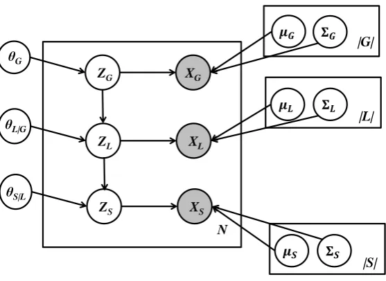
Figure 1: Graphical Representation of the model.
The three types of context feature vectors are formally defined by:
xg =
X
w∈G
I(w)vw (2)
xl =
X
w∈L
I(w)vw (3)
xs=
X
d∈S
I(d)vd (4)
G,LandS are bags of discrete features corresponding to global, local and syntactic context as defined above,wanddare discrete word and dependency context features,vwandvdare embeddings of words and dependency contexts. We also apply L2-normalization to all feature vectors. The weighting by self-information reflects the intuition that rare words are more important for distinguishing senses than common words, and provides an automatic way of filtering the contribution of words without semantic content such as stop-words.
3.2 Probabilistic Generative Model of Context Feature Vectors
We infer the senses of an ambiguous word by combining information provided by the three context feature vectors within a structured generative model. The model assumes that there are three discrete latent variables for each target wordzg,zlandzs, each one generating one of the context feature vectors. The three latent variables form a hierarchical structure, where variables responsible for broader context generate a more context specific latent variable and their corresponding observed feature vector. The density of the context vectors is modelled by Mixtures of Gaussians. The full model is a structured generalization of Gaussian Mixture Models. Sampling context feature vectors follows the generative story:
For each target ambiguous wordn: selectzngvDiscrete(θg)
The corresponding graphical model can be seen in Figure 1. The parameters of the model are:
Θ={θg,θl|g,θs|l,µg,Σg,µl,Σl,µs,Σs} (5)
We constrain the covariance matrices to be diagonal, hence having a smaller number of parameters compared to discrete mixture models for WSI.
3.3 Parameter Estimation
We estimate the parameters of the model by maximum likelihood estimation using the EM algorithm. The equations of E-step and M-step are the following:
E-step
For each samplen∈ {1, .., N}we compute:
γ(Z) =p(Z|X) = Pp(Z,X)
Zp(Z,X)
(6)
Since there are only three dependant latent variables per sample, we can easily compute this step by exact inference.
M-step
We estimate parameters that maximise:
Θnew=E
z|x[arg max
Θnew logp(X,Z|Θ
old)] (7)
Given the factorization implied by the graphical model, each parameter can be estimated independently. The update equations are:
θnew g =
1
N
X
n,l,s
γ(zngls) (8)
θnew l|g =
P
n,sγ(zngls)
P
n,l,sγ(zngls) (9)
θnew s|l =
P
n,lγ(zngls)
P
n,g,sγ(zngls) (10) Updates for means and covariances for thegcontext type are given by:
µnew g =
P
n,l,sγ(zngls)xng
P
n,l,sγ(zngls) (11)
Σnew
g =
P
n,l,sγ(zngls)(xng−µg)(xng−µg)T
P
n,l,sγ(zngls) (12) and similarly for thelandstypes.
We initialize means with the centroids of k-means run independently for each context type, and co-variance matrices with the sample coco-variance.
3.4 Model Selection
One of the most challenging parts of WSI is estimating the number of senses for each ambiguous word type. Since we are working with a probabilistic model we can apply model selection criteria. We use the Integrated Complete Likelihood (ICL) criterion (Biernacki et al., 2000). ICL is a model selection criterion similar to the Bayesian Information Criterion (BIC) (Schwarz, 1978) that seeks a model that provides large evidence for the observed data with a small number of parameters. Following (McLachlan and Peel, 2004) we use the approximation:
ICL(m,X) = logp(X|Θ)−m2k log(N) + X n,g,l,s
wheremkis the total number of parameters to be estimated.
This ICL approximation is exactly equal to BIC additionally penalized by the last term, which is the mean entropy of the distribution of latent variables. The extra penalty term favours models that result in more confident assignments since the entropy of the latent variable distribution will become lower in such cases. This behaviour favours well separated clusters and avoids strongly overlapping components which may be favoured in model selection by BIC. In our experiments, we set|zg|= |zl|= |zs| =K and train models withK in the range of [2, 50]. We observe that given enough training instances, ICL picks models with a large numbers of components corresponding to more fine-grained senses. This is reasonable since with more data the model becomes more confident into making such fine-grained distinctions, and is also likely to encounter unusual word usages.
4 Evaluation
We evaluate our model in two SemEval WSI datasets. For both datasets we parse the data using the Stanford Neural Network dependency parser (Chen and Manning, 2014) using Universal Dependencies (De Marneffe et al., 2014), which is the same format used by the dependency based embeddings. We train a different model for every word type.
4.1 SemEval-2010 Task 14: Word Sense Induction and Disambiguation
The SemEval-2010 WSI dataset consists of 50 verbs and 50 nouns. The task organizers provide a fixed training set with 879,807 instances of the target words. The distribution of instances for each word is highly imbalanced. The test set consists of 8,915 instances. Two types of evaluation are performed: supervised and unsupervised.
The supervised evaluation is performed in two steps. In the first step, a part of the data is used to map the induced sense clusters to a fixed inventory of word senses. In the second step, the fixed sense inventory is used to evaluate the clustering of the rest of the data as a Word Sense Disambiguation system. The reported metric is F-score. Following the task procedures we report two results, one using an 80-20 split of the data for mapping and scoring, and one using a 60-40 split. For both cases, reported results are an average over a 5-fold split.
Unsupervised evaluation for the SemEval task was performed by two clustering quality metrics, V-measure and paired F-score. A problem with clustering evaluation metrics is that they are sensitive to the number of senses (Klapaftis and Manandhar, 2013), with V-measure favouring a high number of senses and F-score the opposite. This behaviour results into ranking two uninformative baselines, 1-cluster-per-instance and most-frequent-sense (or all-in-one), as the best solutions. Li and Titov (2014) argue that for the V-measure, this behaviour can be explained by biases in the estimation of entropy when there is a large number of clusters compared to the number of samples, as is the case in WSI evaluation. They propose the usage of the Best-Upper-Bound (BUB) Entropy Estimator (Paninski, 2003) instead of maximum likelihood estimation that was used by the organizers. They show that the V-measure with the BUB estimator successfully evaluates both uninformative baselines as worse solutions than actual WSI systems. Following this recommendation, we report the V-measure estimated with BUB as the unsupervised evaluation metric.
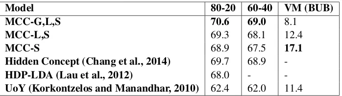
Our default approach for assigning a sense to a word instance is taking the value of p(zs|x) as the probability of a sense being applicable, since it is the variable most directly associated with the am-biguous word. It is possible however, to assign senses to joint configurations of two or all three of the latent variables, in order to better use the information provided by our model. Since the number of pos-sible configurations grows exponentially with the number of latent variables, this approach can lead to very fine-grained partitions of the data. In practice, we observe that only a small number of all these configurations are given a high probability mass. Evaluation results for our model MultiContextContin-uous (MCC) and state-of-the-art systems are reported in Table 2. We report results with both the single variable approach (MCC-S) and joint variable assignments (MCC-L,S and MCC-G,L,S).
Model 80-20 60-40 VM (BUB)
MCC-G,L,S 70.6 69.0 8.1
MCC-L,S 69.3 68.1 12.4
MCC-S 68.9 67.5 17.1
Hidden Concept (Chang et al., 2014) 69.7 68.9
-HDP-LDA (Lau et al., 2012) 68.0 -
[image:7.595.126.475.61.159.2]-UoY (Korkontzelos and Manandhar, 2010) 62.4 62.0 11.4
Table 2: Results on the Semeval-2010 WSI dataset. Dashes indicate that this result was not reported by the authors of the corresponding model. UoY is the best performing model participating in the SemEval-2010 WSI evaluation.
of the sense clusters to the fixed sense inventory and results in the best F-score for the supervised eval-uation. The supervised evaluation benefits from this fine-grained sense distribution since splitting the senses into smaller clusters does not affect the mapping operation, as long as the induced senses are consistent subsets of the gold standard senses. The 60-40 split results into a more difficult mapping problem and can indicate how reliable is the mapping between the sense distribution and the gold stan-dard (Klapaftis and Manandhar, 2013). We see that using the joint configuration of the latent variables again results in the highest F-score, providing evidence of the consistency of the mapping. Contrary to the supervised evaluation, the V-measure favours the clustering provided by thezsvariable alone, since it penalizes the mismatch between the more fine-grained clustering and the gold standard.
4.2 SemEval-2013 Task 13: WSI for graded and non-graded senses.
The SemEval-2013 WSI evaluation dataset consists of 50 word types: 20 verbs, 20 nouns and 10 adjec-tives. There are several differences compared to the SemEval-2010 setting. There are less restriction on the training set, which can be any part or all of the UkWac corpus (Ferraresi et al., 2008). In addition, the test data include instances with multiple applicable senses. There are 4664 instances in the test set, 88.5% of which are labelled with a single sense, 11% labelled with two senses and 0.5% with three. Systems are asked to provide an estimate of the applicability of each sense.
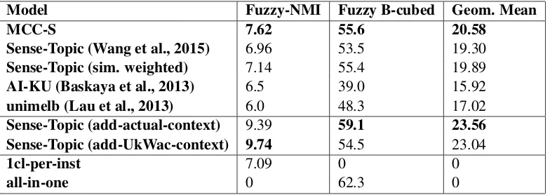
The evaluation metrics also differ from those of SemEval-2010, in order to cope with the multiple sense labelling. Clustering evaluation is performed with the Fuzzy B-cubed and Fuzzy normalized Mu-tual Information (NMI) criteria. Fuzzy NMI favours solutions with many clusters giving a high score to the 1-cluster-per-instance baseline, while Fuzzy B-cubed favours few clusters and favours the all-in-one baseline. Following (Wang et al., 2015), we use those two metrics but also report the geometric mean of the two, which provides a more balanced metric and also assigns a score of zero to both the uninfor-mative baselines. We use the top 3 most probable assignments of thezsvariable with the corresponding probability as the applicability weight. Results can be seen in Table 3.
Model Fuzzy-NMI Fuzzy B-cubed Geom. Mean
MCC-S 7.62 55.6 20.58
Sense-Topic (Wang et al., 2015) 6.96 53.5 19.30
Sense-Topic (sim. weighted) 7.14 55.4 19.89
AI-KU (Baskaya et al., 2013) 6.5 39.0 15.92
unimelb (Lau et al., 2013) 6.0 48.3 17.02
Sense-Topic (add-actual-context) 9.39 59.1 23.56
Sense-Topic (add-UkWac-context) 9.74 54.5 23.04
1cl-per-inst 7.09 0 0
[image:8.595.105.497.62.201.2]all-in-one 0 62.3 0
Table 3: Results on the SemEval-2013: Task 13 dataset. All Sense-Topic model variants are reported from (Wang et al., 2015). Results with extra context (add-actual-context, add-UkWac-context) do not use the same evaluation setting and are not directly comparable to the rest. AI-KU and unimelb are systems participating in the SemEval-2013 evaluation.
5 Discussion
We attribute the good performance of the proposed model to its capacity to handle data sparsity. Both the multiple context representations and the usage of low dimensional feature embeddings contribute towards that goal. The importance of dealing with sparse inputs can be seen from the generally good performance of Bayesian latent variable models for WSI (Wang et al., 2015; Chang et al., 2014) . While these models manage to deal with the sparsity of words, they still do not manage to effectively utilize syntactic features as we do with dependency feature embeddings. By using pretrained embeddings our model has access to a very large feature set (about 220k words and 1.3m dependency context features), while having to estimate a relatively small number of parameters. In Table 4, we show some examples where clusters are formed by different but semantically related words, and the importance of syntactic features.
A weakness of the proposed model is that context representations corresponding to senses are assumed to follow Gaussian distributions. We cannot expect this assumption to hold in general, but our evaluation suggests that it is a reasonable approximation. It is possible to extend the model by using a separate Mixture of Gaussians to model each individual sense. While this extension would provide additional capacity to the model for modelling sense specific contextual representations with complex probability densities, it can lead to parametric explosion and severe overfitting.
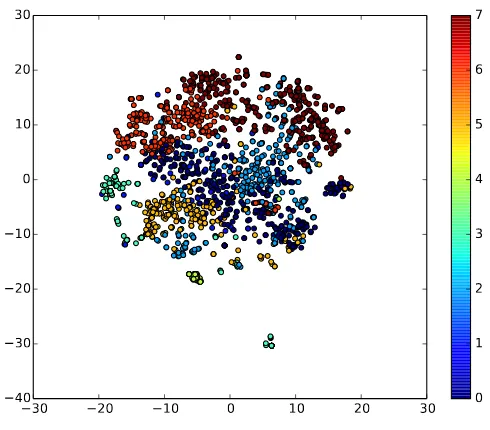
In Figure 2, we use t-SNE (Maaten and Hinton, 2008) to visualize the syntactic context vectors of the word “operate” from the SemEval-2010 training data and their sense assignments. We see that clustered points generally form compact groups, though they are not clearly separated. In order to model senses with contexts that do not follow a Gaussian distribution, the model favours additional clusters. In practice, we observe that this behaviour does not pose a significant problem as long as these finer-grained clusters are consistent with the underlying sense distribution, which was shown by the supervised evaluation of SemEval-2010. If a coarse grained distribution is desired, methods that merge Gaussian components as a postprocessing step could be considered (Hennig, 2010).
6 Conclusion
30 20 10 0 10 20 30 40
30 20 10 0 10 20 30
[image:9.595.163.408.79.294.2]0 1 2 3 4 5 6 7
Figure 2: 2-d t-SNE of the syntactic context vectors of the word “operate”. Different colours correspond to different cluster assignments. Best viewed in colour.
Cluster 6
... energy-efficient appliances and how tooperatethem efficiently ...
... temperature rises enough for the heat pump tooperatemore efficiently than your old furnace ... ... software to enable users tooperatetheir computers remotely ...
Cluster 5
... 44 of these storesoperateas monro muffler brake & service ...
... many industries with volatile profits ranging from oil exploration to computer softwareoperatewithout substantial government regulation ...
... bfx hospitality group , inc. owns andoperatesfood services ...
Table 4: Instances of “operate” belonging into two different clusters. The contexts do not share many common words, but they are semantically related. The second instance of cluster 5 shares words with the third instance of cluster 6 (“software”, “computer”), but is assigned the correct sense because the syntactic features indicate the long range subject dependency with “industries”.
Criterion. We evaluate our model in two competitive WSI benchmarks, achieving state-of-the-art results.
Acknowledgements
Alexandros Komninos was supported by EPSRC via an Engineering Doctorate in LSCITS. Suresh Man-andhar was supported by EPSRC grant EP/I037512/1, A Unified Model of Compositional & Distribu-tional Semantics: Theory and Application.
References
Osman Baskaya, Enis Sert, Volkan Cirik, and Deniz Yuret. 2013. Ai-ku: Using substitute vectors and co-occurrence modeling for word sense induction and disambiguation. pages 300–306.
[image:9.595.78.524.360.484.2]David M Blei, Andrew Y Ng, and Michael I Jordan. 2003. Latent dirichlet allocation. Journal of machine Learning research, 3(Jan):993–1022.
Samuel Brody and Mirella Lapata. 2009. Bayesian word sense induction. InProceedings of the 12th Conference of the European Chapter of the Association for Computational Linguistics, pages 103–111. Association for Computational Linguistics.
Baobao Chang, Wenzhe Pei, and Miaohong Chen. 2014. Inducing word sense with automatically learned hidden concepts. InCOLING, pages 355–364.
Danqi Chen and Christopher D Manning. 2014. A fast and accurate dependency parser using neural networks. In Proceedings of the 2014 Conference on Empirical Methods in Natural Language Processing (EMNLP), volume 1, pages 740–750.
Ronan Collobert, Jason Weston, L´eon Bottou, Michael Karlen, Koray Kavukcuoglu, and Pavel Kuksa. 2011. Natural language processing (almost) from scratch.The Journal of Machine Learning Research, 12:2493–2537. Marie-Catherine De Marneffe, Timothy Dozat, Natalia Silveira, Katri Haverinen, Filip Ginter, Joakim Nivre, and Christopher D Manning. 2014. Universal stanford dependencies: A cross-linguistic typology. InProceedings of LREC, pages 4585–4592.
Antonio Di Marco and Roberto Navigli. 2013. Clustering and diversifying web search results with graph-based word sense induction.Computational Linguistics, 39(3):709–754.
Adriano Ferraresi, Eros Zanchetta, Marco Baroni, and Silvia Bernardini. 2008. Introducing and evaluating ukwac, a very large web-derived corpus of english. InProceedings of the 4th Web as Corpus Workshop (WAC-4) Can we beat Google, pages 47–54.
Christian Hennig. 2010. Methods for merging gaussian mixture components. Advances in data analysis and classification, 4(1):3–34.
Yanzhou Huang, Deyi Xiong, Xiaodong Shi, Yidong Chen, ChangXing Wu, and Guimin Huang. 2016. Adapted competitive learning on continuous semantic space for word sense induction. Neurocomputing, 171:1475–1485. Ignacio Iacobacci, Mohammad Taher Pilehvar, and Roberto Navigli. 2015. Sensembed: learning sense
embed-dings for word and relational similarity. InProceedings of ACL, pages 95–105.
David Jurgens and Ioannis Klapaftis. 2013. Semeval-2013 task 13: Word sense induction for graded and non-graded senses. InSecond joint conference on lexical and computational semantics (* SEM), volume 2, pages 290–299.
Ioannis P Klapaftis and Suresh Manandhar. 2010. Word sense induction & disambiguation using hierarchical random graphs. InProceedings of the 2010 conference on empirical methods in natural language processing, pages 745–755. Association for Computational Linguistics.
Ioannis P Klapaftis and Suresh Manandhar. 2013. Evaluating word sense induction and disambiguation methods.
Language resources and evaluation, 47(3):579–605.
Alexandros Komninos and Suresh Manandhar. 2016. Dependency based embeddings for sentence classification tasks. InProceedings of NAACL:HLT, pages 1490–1500. Association for Computational Linguistics.
Ioannis Korkontzelos and Suresh Manandhar. 2010. Uoy: Graphs of unambiguous vertices for word sense in-duction and disambiguation. InProceedings of the 5th international workshop on semantic evaluation, pages 355–358. Association for Computational Linguistics.
Jey Han Lau, Paul Cook, Diana McCarthy, David Newman, and Timothy Baldwin. 2012. Word sense induction for novel sense detection. InProceedings of the 13th Conference of the European Chapter of the Association for Computational Linguistics, pages 591–601. Association for Computational Linguistics.
Jey Han Lau, Paul Cook, and Timothy Baldwin. 2013. unimelb: Topic modelling-based word sense induction for web snippet clustering. InProceedings of the 7th International Workshop on Semantic Evaluation (SemEval 2013), pages 217–221.
Omer Levy and Yoav Goldberg. 2014. Dependency-based word embeddings. In Proceedings of ACL, pages 302–308.
Laurens van der Maaten and Geoffrey Hinton. 2008. Visualizing data using t-sne. Journal of Machine Learning Research, 9(Nov):2579–2605.
Suresh Manandhar, Ioannis P Klapaftis, Dmitriy Dligach, and Sameer S Pradhan. 2010. Semeval-2010 task 14: Word sense induction & disambiguation. InProceedings of the 5th international workshop on semantic evaluation, pages 63–68. Association for Computational Linguistics.
Geoffrey McLachlan and David Peel. 2004.Finite mixture models. John Wiley & Sons.
Tomas Mikolov, Ilya Sutskever, Kai Chen, Greg S Corrado, and Jeff Dean. 2013. Distributed representations of words and phrases and their compositionality. In Advances in neural information processing systems, pages 3111–3119.
Roberto Navigli. 2009. Word sense disambiguation: A survey.ACM Computing Surveys (CSUR), 41(2):10. Arvind Neelakantan, Jeevan Shankar, Alexandre Passos, and Andrew McCallum. 2015. Efficient non-parametric
estimation of multiple embeddings per word in vector space. arXiv preprint arXiv:1504.06654.
Liam Paninski. 2003. Estimation of entropy and mutual information. Neural computation, 15(6):1191–1253. Gideon Schwarz. 1978. Estimating the dimension of a model. The annals of statistics, 6(2):461–464.
Yee Whye Teh, Michael I Jordan, Matthew J Beal, and David M Blei. 2012. Hierarchical dirichlet processes.
Journal of the american statistical association.
Joseph Turian, Lev Ratinov, and Yoshua Bengio. 2010. Word representations: a simple and general method for semi-supervised learning. InProceedings of the 48th annual meeting of the association for computational linguistics, pages 384–394. Association for Computational Linguistics.