Improving a Neural-based Tagger for Multiword Expression Identification
Duˇsan Variˇs, Natalia Klyueva
Institute of Formal and Applied Linguistics, Charles University; The Hong Kong Polytechnic University Malostransk´e n´amˇest´ı 25, Prague; 11 Yuk Choi Rd, Hung Hom,
[email protected], [email protected]
Abstract
In this paper, we present a set of improvements introduced to MUMULS, a tagger for the automatic detection of verbal multiword expressions. Our tagger participated in the PARSEME shared task and it was the only one based on neural networks. We show that character-level embeddings can improve the performance, mainly by reducing the out-of-vocabulary rate. Furthermore, replacing the softmax layer in the decoder by a conditional random field classifier brings additional improvements. Finally, we compare different context-aware feature representations of input tokens using various encoder architectures. The experiments on Czech show that the combination of character-level embeddings using a convolutional network, self-attentive encoding layer over the word representations and an output conditional random field classifier yields the best empirical results.
Keywords:multiword expressions, machine learning, deep learning, conditional random field
1.
Introduction
Multiword Expression (MWE) is a sequence of words for which the meaning of a whole sequence cannot be derived from the meaning of its components straightforwardly. MWEs are viewed by computational linguists as a “pain in the neck of NLP” due to their non-compositionality and irregularity that can cause problems in areas such as ma-chine translation, terminology extraction, etc. Regarding this, MWEs are largely addressed in both the theoretical and applied research. Associative measures (calculating association between distinct words in MWE) are usually used for extracting MWEs (Ramisch, 2015; Kilgarriff et al., 2014). The identification of MWE in the text is thus a challenging task.
Within PARSEME’s special MWE-related project1, re-searchers from different countries created guidelines on how to define MWEs in the text and annotated corpora in 18 languages. The focus was on verbal MWEs which were categorized into five classes: idioms (ID), light verb con-structions (LVC), inherently reflexive verbs (IReflV), verb-particle constructions (VPC), and other (OTH). The process of annotation was language-dependent. For instance, in Hungarian, VPCs are annotated and IReflVs are not, how-ever, in Czech it is the other way around.
These data then served as the training data for systems par-ticipating in the shared task on automatic verbal multiword expression (VMWE) identification (Savary et al., 2017). In addition to the MWEs markings, morphosyntactic mark-ings were provided in the corpora as well.
Seven systems based on various approaches and algorithms participated in the task. Two of them were based on condi-tional random field (CRF) (Maldonado et al., 2017; Boros¸ et al., 2017), the other was trained using dependency pars-ing (Simk´o et al., 2017) and the winner was a transition-based system exploiting syntactic rules (Al Saied et al., 2017).
For some of the languages, our previous model based on the neural networks (NN) had comparable scores with other
1https://typo.uni-konstanz.de/parseme/
multilingual systems, yet it performed best only in one lan-guage – Romanian. Later comparison between our system and the winner (transition-based approach) revealed a large gap between the MWE-based scores, which focus on exact matches between the hypothetical and the gold MWEs and the token-based scores, which compare individual tokens from the MWEs. Our approach does not perceive MWEs as a whole, labeling each token individually, although, some-times it can capture long distant dependencies between the MWE components.
In this paper, we describe our ongoing work on improv-ing our tagger, MUMULS, usimprov-ing the current state-of-the-art sequence-to-sequence techniques applied in other NLP tasks, including different styles of embedding of the input tokens, creating a context-aware feature representation of the input sequence and generating of the target labels. This paper is structured as follows. We describe the data preprocessing in Section 2. In Section 3., we describe the proposed improvements. In Section 4., we describe the ex-periments and analyze their results. We conclude our find-ings in Section 5.
2.
Data Preparation
The training data were provided in two files per each lan-guage, one in the CoNLL-U format with the morphosyntac-tic annotations and the other in a specially created parseme TSV format with the respective annotations of VMWEs. From these two files, we extract word forms, lemmas, part-of-speech (POS) tags and target MWE labels and use them to train our models.
The MWE labels have a following format: “mwe id”:“mwe label” (e.g. 1:ID), where “mwe id” is used to distinguish different MWEs within the same sentence. A single token can also belong to multiple MWEs having multiple labels separated by a semicolon (e.g.1:ID;2:IReflV).
without the “mwe id”2 and the following tokens receive a specialCONT label. During the postprocessing, we as-sign an unique “mwe id”to each label except forCONT and replace each of the following CONT labels with the same “mwe id”. If the first label encountered in the la-beled sequence isCONT, we use the most frequent MWE label (based on the training data) to replace it.
Below is an excerpt from the training file for French with an idiomatic expressionmettre un terme– ‘finish’ (the fourth and fifth column contain original and preprocessed labels respectively):
Il il PRON _ _
met mettre VERB 1:ID ID
un un DET 1 CONT
terme terme NOUN 1 CONT
`
a `a ADP _ _
sa son DET _ _
carri`ere carri`ere NOUN _ _
Clearly, our processing methods cannot handle several phe-nomena, for example, crossing MWEs or tokens that belong to multiple MWEs. For this reason, we used an “Oracle” tagger that only applied preprocessing and postprocessing on the gold labels in the test data and compared the pro-duced output with the original labels. The results showed that using our processing methods can still produce a tagger with an f-measure score of 0.95 and higher. Therefore, we consider the suggested processing methods sufficient for this task.
3.
System Description
Our MWE tagger is a sequence classifier that predicts the target labels using feature representations computed by a deep neural network (DNN). In the last few years, DNNs started achieving the state-of-the-art results in many NLP tasks including machine translation (Sutskever et al., 2014), natural language generation (Wen et al., 2015) and more importantly POS tagging (P´erez-Ortiz and Forcada, 2001) and named entity recognition (Lample et al., 2016). The system we submitted to the VMWE shared task 3 was implemented using the TensorFlow4 open source library (Abadi et al., 2016). However, our current research-in-progress is implemented in the Neural Monkey5(Helcl and Libovick´y, 2017) framework for sequence modeling, be-cause it enables easier prototyping and replication of the experiments.6
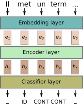
Figure 1 shows a general overview of the system architec-ture. It consists of three separate layers, the embedding layer, which assigns an embedding vector to each input
2In the case of multiple MWE labels, the token receives only
the first one. 6The code used during experiments together with
the experiment configurations is available at https: //github.com/ufal/neuralmonkey/tree/lrec_
Classifier layer
e1 e2 e3 e4 e5
h1 h2 h3 h4 h5
Figure 1: General overview of the MUMULS MWE tagger.
eirepresents the embedding of the i-th word,hirepresents
its context-aware representation.
token, the encoder layer, which transforms each embed-ding vector to a context-aware vector representation and the classifier layer, which assigns an output label to each token based on the context-aware representation. We de-scribe each layer in more detail in the following sections.
3.1.
Embedding Layer
The role of the embedding layer is to assign each wordwiin
the input sequencew= (w1, .., wn)an embedding vector ei∈Rdwheredis the embedding size, creating a sequence
representatione= (e1, .., en). We can accomplish this in
two ways: either by using an embedding lookup table or by computing the embedding using the embeddings of its characters. We call the former methodword-level embed-dingand the latter acharacter-level embedding.
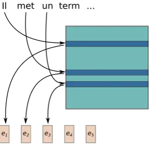
Figure 2 illustrates an embedding assignment using the bedding lookup table. Each word is mapped to an em-bedding based on its vocabulary index. OOV words are mapped to a special “UNK” embedding. The poor handling of OOV words and the size of the embedding lookup table are the main issues when using the word-level embeddings and can be eliminated to a certain degree by the character-level embeddings.
3.1.1. Character-level embeddings
Character-level embeddings are word representations cre-ated by combining the embeddings of the characters in the word. To capture dependencies between the characters in the word, we use either a recurrent neural network (RNN) or a convolutional neural network (CNN).
Figure 2 shows the process of creating the character-level embedding using the RNN. A sequence of embedded char-acters ch = (ch1, .., chn), chi ∈ Rdch, which is cre-ated using an embedding lookup table similar to the word-level embedding method, is fed to the bidirectional RNN (BiRNN) (Graves and Schmidhuber, 2005). The BiRNN creates a context-aware representation of each character h = (h1, .., hn),7 hi ∈ Rdh in a recurrent fashion using
7
Il met un term ...
e1 e2 e3 e4 e5
Figure 2: A word-level embedding example. Every input word is assigned an embedding depending on its vocabu-lary index.
t
e
r
m
e
e p o o l i n g
Figure 3: An illustration of the character-level RNN em-bedding. The outputs from each step of the BiRNN are concatenated and the whole output sequence is pooled to create the embedding of the word. The embeddings of the individual characters are omitted for simplicity.
the following formula:
hi=f(hi−1, chi) (1)
The function f(h, ch) is computed by a recurrent cell, usually the Long-Short Term Memory (LSTM) (Hochre-iter and Schmidhuber, 1997) or the Gated Recurrent Unit (GRU) (Chung et al., 2014). After we get the context-aware representation of each character, we apply pooling (maxi-mum or average) over the whole sequencehto get the em-bedding of the word.
Initially created and applied in image recognition task, CNNs became popular in the NLP tasks as well. The method relies on kernel sliding, however, the kernel slides over the sequence of embedded characters instead of image pixels. The Figure 4 shows the architecture of the CNN that can be used to create character-level embeddings. We apply a set of filtersF = [f ilt1, .., f iltk]on the sequence
of embedded characters. A filterf iltj of widthltakes an
inputX ∈ Rl×dch and transforms it into a single output Y ∈ Rd/|F|, wheredis again the size of the output word
embedding. We pad the sequence of characters to make
for eachi, created by the forward and backward run respectively. The states are concatenated to create the representationhi
t
e
r
m
e
e p o o l i n g
Figure 4: An illustration of the character-level convolu-tional embedding. The sequence of characters is padded to guarantee equal length of the filter outputs. We omit the embeddings of the individual characters for simplicity.
h2 h3 h4 h5 h1
e2 e3 e4 e5 e1
Figure 5: An illustration of the BiRNN encoder. Each em-beddingeiis pasted to the RNN cell to produce a
context-aware representationhi.
each filter produce a sequence of the same length. These output sequences are then concatenated element-wise to produce a single sequenceh = (h1, ..hn)and a we apply
pooling to produce the embedding of the word.
To provide additional information for the tagger, we encode not only the word forms but also lemmas and POS tags that are available in the training data. For each token, we en-code its word form, lemma and POS tag using a separate embedding lookup table in case of the word-level embed-ding and a separate character-level encoder in case of the character-level embedding. The resulting embeddings of the word form, lemma and POS tag are then concatenated to create the embedding of the token.
3.2.
Encoder Layer
The purpose of the encoder layer is to take the embed-dings of the words e = (e1, .., en) provided by the
em-bedding layer and transform them to a representationh = (h1, .., hn)where each embedding hi contains additional
information about its neighbors. We examine three meth-ods of doing so: using a BiRNN, a deep convolutional net-work and a self-attentive netnet-work.
Figure 5 shows the architecture of the BiRNN encoder. The process is similar to the character-level BiRNN encoder: the input embeddingseare transformed tohusing the fol-lowing formula:
hi=f(hi−1, ei) (2)
h2 h3 h4 h5
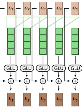
Figure 6: An illustration of the deep convolutional encoder with depth 1. The filter creates an itermediate embedding with double of the original embedding size and the GLU gating mechanism reduces the embedding back to the orig-inal size. Residual connections are applied to allow deep convolutions. The output of the layer can be used as input to another layer.
Figure 7: A simplified illustration of a single self-attentive layer consisting of a multi-head attention and feed forward sublayer. After each sublayer, residual connections and a layer normalization are applied. The layers can be stacked to create a deeper architecture.
Figure 6 describes the deep convolutional encoder architec-ture first used by a Facebook machine translation system (Gehring et al., 2017). In contrast to the RNN, convolu-tions do not provide explicit way to encode the position of a word in the input sequence. To counter this, we add ad-ditional positional information to the embeddings (Gehring et al., 2017; Vaswani et al., 2017). The position-aware em-beddings are then transformed using a filter F ∈ R2d×ld,
wherel is the width of the filter. The filter takes l input embeddings and transforms them into a single output em-beddingh0 ∈ R2d. A Gated Linear Unit (GLU) (Dauphin
et al., 2016), is applied on theh0as a gating mechanism to introduce non-linearity, producingh ∈ Rd. We also add
residual connections (He et al., 2016) to the output of the GLU to enable deep convolutions. These convolutional lay-ers can be stacked one on top of another producing deeper representations. We use the output from the last layer as the
MWE-based F1 token-based F1
word-lvl 0.42 0.57
Table 1: Comparison between different embedding meth-ods.
MWE-based F1 token-based F1
birnn-softmax 0.69 0.78
Table 2: Comparison between different encoder architec-tures and output classifiers.
input for the classifier layer.
The structure of the self-attentive encoder (Vaswani et al., 2017) is described in Figure 7. Similar to the convolu-tional encoder, the self-attentive encoder does not explic-itly capture information about the position of the input in the sequence. Therefore, we use the position-aware em-beddings again. We apply a multi-head attention mech-anism on these embeddings (Vaswani et al., 2017) and a position-wise fully-connected layer. After each sublayer, a layer normalization (Ba et al., 2016) and a residual con-nections are added. Again, the process can be repeated by stacking multiple layers using the output of the previous layer as the input of the following one. We pass the output of the last layer to the classifier layer.
3.3.
Classifier Layer
The classier layer takes the output representations h = (h1, .., hn)produced by the encoder layer and uses them
to predict the target sequence. We compare two methods: a softmax classifier and a CRF classifier.
The softmax classifier first transforms each hidden repre-sentationhi into a vector of logits yi ∈ R|V|, where|V|
is the size of the target vocabulary. The logits y are then normalized using a softmax function creating a distribution over the target vocabulary. During training, we minimize the cross-entropy between the output distribution and the gold labels. During the inference, a label with the highest probability is selected.
System MWE F1 token F1 System MWE F1 token F1
BG
MUMULS-old 0.34 0.59
LT MUMULS-old 0.00 0.00
MUMULS 0.50 0.62 MUMULS 0.19 0.25
PARSEME winner 0.61 0.66 PARSEME winner 0.28 0.25
CS
MUMULS-old 0.16 0.23
PT MUMULS-old 0.44 0.60
MUMULS 0.67 0.73 MUMULS 0.40 0.52
PARSEME winner 0.71 0.73 PARSEME winner 0.67 0.71
DE
MUMULS-old 0.21 0.34
RO MUMULS-old 0.77 0.84
MUMULS 0.33 0.40 MUMULS 0.66 0.71
PARSEME winner 0.41 0.45 PARSEME winner 0.77 0.84
FR
MUMULS-old 0.09 0.29
SL MUMULS-old 0.31 0.45
MUMULS 0.38 0.48 MUMULS 0.32 0.40
PARSEME winner 0.51 0.61 PARSEME winner 0.43 0.47
IT
MUMULS-old – –
TR MUMULS-old 0.34 0.45
MUMULS 0.07 0.07 MUMULS 0.40 0.48
PARSEME winner 0.40 0.44 PAESEME winner 0.55 0.55
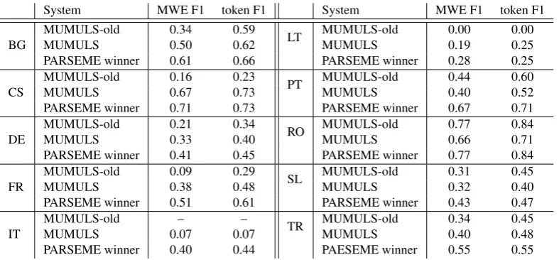
Table 3: Comparison between our best systems configuration, old MUMULS system performance and the best submitted system across languages participating in the PARSEME Shared Task.
CRF classifer tries to minimize the negative log-likelihood of the gold target sequence y = (y1, .., yn) based on the between the labels computed using transition parameters
θ∈R|V|x|V|, where|V|denotes the size of the target label
vocabulary. During the inference, the CRF classifier uses the Viterbi decoding algorithm (Forney, 1973) to output the sequence with the highest score.
4.
Experiments
When we evaluated the suggested system configurations, we compared each layer configurations separately. We used the Czech dataset available for the PARSEME shared task. We used the MWE-based F1 measure metric to evaluate the performance of each system configuration. The metric is a standard F1 measure based on the precision and recall of the evaluated systems. For each MWE (represented as a set of word indices) in the reference, it searches for exact matches in the predicted MWEs. For comparison, we also used a fuzzy, token-based F1 measure which allows partial matches between the gold and predicted MWEs.
First we compared the variants of the embedding layer. We used the embedding size 100 for each word form, lemma and POS tag, resulting in a token embedding size 300. We fixed the encoder layer to a BiRNN with the hidden state size 300 and an LSTM recurrent cell. We only used the softmax classifier during this comparison. All experi-ments had a fixed dropout of 0.8. The word-level embed-ding method used a separate vocabularies for word forms, lemmas and POS tags. The character-level embeddings used the same character vocabulary for each factor. In the character-level RNN embedding, we set the size of the hid-den state to the size of the input embedding. We compared the performance of both LSTM (char-rnn-lstm) and GRU
(char-rnn-gru) cell. In the character-level CNN (char-conv), we tried sets of filters of lengths ranging from 2 to 5 and 2 to 6 respectively. In both character-level embedding meth-ods, we compared both maximum (max) and average (avg) pooling.
Table 1 shows the individual performance of each embed-ding method. First, we can see that using the character-level embeddings brings significant improvement over the word-level embeddings. Second, the choice of the RNN cell seems to have little to no impact on the performance of the char-rnn embedding method. Finally, the results show that the char-conv embedding method yields the best results and that the maximum pooling method outperforms the av-erage pooling.
Next, we compared the suggested encoder layer configura-tions. We used the convolutional character-level CNN with maximum pooling for embedding layer. The BiRNN on the encoder layer was identical to the one used during the embedding layer comparison. The deep convolutional en-coder (deep-convo) had three layers, each having the filter width 3. The self-attention encoder (self-att) also had three layers, each having 10 attention heads and a feed-forward network with the hidden size 450. We chose the parameters so that each model had a comparable number of trainable variables. For each encoder, the size of the output hidden states was identical to the size of the input embeddings. We compared both the softmax and CRF classifier with each encoder.
Table 2 compares the performance of each encoder ar-chitecture and classifier method. The self-attention en-coder achieved the best results being slightly better than the BiRNN encoder. The results also show that replacing the softmax layer with the CRF classifier consistently im-proves the performance.
of the models with the results reported in the shared task. We can see, that our improvements were reflected in the MUMULS performance when compared with our old sub-mission. However, we still were not able to beat the best submission. The lower performance of the improved MU-MULS on the Romanian requires additional investigation in the future.
5.
Conclusion
We described an ongoing work on improving MUMULS, a neural-based system for automatic identification of ver-bal multiword expressions. We compare several state-of-the-art architectures, experiment with different embedding methods and implement sequence model for label predic-tion using CRF. The results show that for most of the lan-guages, our modifications bring additional boost in the sys-tem performance.
In the future, we plan to further investigate the possibili-ties of scaling the presented architectures and studying the model capacities with respect to the provided data. Special attention will be focused on investigating the decrease in performance for the Romanian because it is a language in which the old version of MUMULS yielded the best results.
6.
Acknowledgements
The first author has been supported by the LIN-DAT/CLARIN project of the Ministry of Education, Youth and Sports of the Czech Republic (projects LM2015071 and OP VVV VI CZ.02.1.01/0.0/0.0/16 013/0001781), by the Charles University SVV project number 260 453 and by the Meta-Net/T4ME Net project of the European Union (project FP7-ICT-2009-4-249119).
The second author has been supported by the postdoctoral fellowship grant of the Hong Kong Polytechnic University, project code G-YW2P.
7.
Bibliographical References
Abadi, M., Agarwal, A., Barham, P., Brevdo, E., Chen, Z., Citro, C., Corrado, G. S., Davis, A., Dean, J., Devin, M., et al. (2016). Tensorflow: Large-scale machine learn-ing on heterogeneous distributed systems. arXiv preprint arXiv:1603.04467.
Al Saied, H., Constant, M., and Candito, M. (2017). The ATILF-LLF System for Parseme Shared Task: a Transition-based Verbal Multiword Expression Tagger. InProceedings of the 13th Workshop on Multiword Ex-pressions (MWE 2017), pages 127–132, Valencia, Spain, April. Association for Computational Linguistics. Ba, L. J., Kiros, R., and Hinton, G. E. (2016). Layer
nor-malization.CoRR, abs/1607.06450.
Boros¸, T., Pipa, S., Barbu Mititelu, V., and Tufis¸, D. (2017). A data-driven approach to verbal multiword expression detection. PARSEME Shared Task system description paper. In Proceedings of the 13th Workshop on Multi-word Expressions (MWE 2017), pages 121–126, Valen-cia, Spain, April. Association for Computational Lin-guistics.
Chung, J., Gulcehre, C., Cho, K., and Bengio, Y., (2014). Empirical evaluation of gated recurrent neural networks on sequence modeling.
Dauphin, Y. N., Fan, A., Auli, M., and Grangier, D. (2016). Language modeling with gated convolutional networks. arXiv preprint arXiv:1612.08083.
Forney, G. D. (1973). The viterbi algorithm. Proc. of the IEEE, 61:268 – 278, March.
Gehring, J., Auli, M., Grangier, D., Yarats, D., and Dauphin, Y. (2017). Convolutional sequence to se-quence learning.
Graves, A. and Schmidhuber, J. (2005). Framewise Phoneme Classification with Bidirectional LSTM and other Neural Network Architectures. Neural Networks, 18(5):602–610.
He, K., Zhang, X., Ren, S., and Sun, J. (2016). Deep residual learning for image recognition. In 2016 IEEE Conference on Computer Vision and Pattern Recogni-tion, CVPR 2016, Las Vegas, NV, USA, June 27-30, 2016, pages 770–778. IEEE Computer Society.
Helcl, J. and Libovick´y, J. (2017). Neural Monkey: An Open-source Tool for Sequence Learning. The Prague Bulletin of Mathematical Linguistics, 107:5–17.
Hochreiter, S. and Schmidhuber, J. (1997). Long short-term memory. Neural Comput., 9(8):1735–1780, November.
Kilgarriff, A., Baisa, V., Buˇsta, J., Jakub´ıˇcek, M., Kov´aˇr, V., Michelfeit, J., Rychl´y, P., and Suchomel, V. (2014). The sketch engine: ten years on. Lexicography, pages 7–36. Lample, G., Ballesteros, M., Subramanian, S., Kawakami,
K., and Dyer, C. (2016). Neural architectures for named entity recognition. In Kevin Knight, et al., editors, HLT-NAACL, pages 260–270. The Association for Computa-tional Linguistics.
Maldonado, A., Han, L., Moreau, E., Alsulaimani, A., Chowdhury, K. D., Vogel, C., and Liu, Q. (2017). De-tection of Verbal Multi-Word Expressions via Condi-tional Random Fields with Syntactic Dependency Fea-tures and Semantic Re-Ranking. InProceedings of the 13th Workshop on Multiword Expressions (MWE 2017), pages 114–120, Valencia, Spain, April. Association for Computational Linguistics.
P´erez-Ortiz, J. A. and Forcada, M. L. (2001). Part-of-speech tagging with recurrent neural networks. In Pro-ceedings of the International Joint Conference on Neural Networks, IJCNN 2001, pages 1588–1592.
Ramisch, C. (2015). Multiword Expressions Acquisition: A Generic and Open Framework, volume XIV of The-ory and Applications of Natural Language Processing. Springer.
Sutskever, I., Vinyals, O., and Le, Q. V. (2014). Sequence to sequence learning with neural networks. In Proceed-ings of the 27th International Conference on Neural In-formation Processing Systems, NIPS’14, pages 3104– 3112, Cambridge, MA, USA. MIT Press.
Vaswani, A., Shazeer, N., Parmar, N., Uszkoreit, J., Jones, L., Gomez, A. N., Kaiser, L., and Polosukhin, I. (2017). Attention is all you need.