Improved Transductive Learning
Zhu Zhang
School of Information and Department of EECS, University of Michigan, Ann Arbor, MI 48105, U.S.A
Abstract. This paper studies the problem of mining relational data hidden in natural language text. In particular, it approaches the relation classification problem with the strategy of transductive learning. Dif-ferent algorithms are presented and empirically evaluated on the ACE corpus. We show that transductive learners exploiting various lexical and syntactic features can achieve promising classification performance. More importantly, transductive learning performance can be significantly im-proved by using an induced similarity function.
1
Introduction
The world today is full of various information sources, with different ways of representing the same information. One common problem that arises in the data management community is that data existing in one format may be needed in a different format for another purpose. An instance of this general problem is that relational data don’t always exist in the form of relational tables; lots of them are hidden in natural language text. For example, (author, book) pairs can be instantiated as “. . .Shakespeare’s famous workHamlet . . . ” or “. . .A Brief History of Timewas written byStephen Hawking. . . ” in text.
On the other hand, within the information retrieval and natural language processing community, Information Extraction (IE) systems are understood as techniques for automatically extracting information from text, specifically, iden-tifying relevant information (usually of pre-defined types) from text documents in a certain domain. Once extracted, the information can be used for purposes such as database population and text indexing. While significant progress has been made in IE research, stimulated in particular by the Message Understand-ing Conferences (MUC)1 and the recent ACE (Automatic Content Extraction) program2 organized by the LDC (Linguistic Data Consortium), it is generally agreed that many barriers exist to the wider use of IE technologies due to the difficulties in adapting systems to new applications and domains. Keeping track of dynamic information sources (e.g., web pages) is challenging as well.
To address these challenges, there has been a recent trend shift in the research community from knowledge-based approaches to machine learning techniques. Moreover, due to the cost related to acquiring large amount of labeled training
1 http://www.itl.nist.gov/iaui/894.02/related projects/muc/ 2
http://www.ldc.upenn.edu/Projects/ACE/
R. Dale et al. (Eds.): IJCNLP 2005, LNAI 3651, pp. 402–413, 2005. c
data, researchers have been looking at various learning algorithms exploiting cheaply available unlabeled data (usually in much larger amounts), which aim at minimizing the need for labeled data while still achieving comparable results. According to the scope of ACE, current IE research has three main objectives: Entity Detection and Tracking (EDT), Relation Detection and Characterization (RDC), and Event Detection and Characterization (EDC). This study focuses on the second subproblem, RDC. In particular, the goal is to automatically classify binary relations between entities, i.e., to decide in which relational table to put each entity pair, using transductive learning algorithms. We propose an improved transductive learner and empirically compare it with the baseline learner on the ACE corpus.
2
Related Work
The current paper draws upon previous work in NLP and machine learning.
2.1 Relation Extraction and Classification
Within the realm of information extraction, there are several representative sys-tems that use machine learning for extracting relations.
Snowball [1] is a bootstrapping-based system that requires only a handful of training examples of tuples of interest. These examples are used to generate extraction patterns, which in turn result in new tuples being extracted from the document collection. At each iteration of the extraction process, Snowball evaluates the quality of these patterns and tuples without human intervention, and keeps only the most reliable ones for the next iteration. A scalable evaluation methodology is also developed for the task. The approach was illustrated on the problem of extracting (organization, headquarter location)pairs from a collection of more than 300,000 newspaper documents.
DIPRE (Dual Iterative Pattern Relation Expansion) [2] is another technique that exploits the duality between sets of patterns and relations to grow the target relation starting from a small sample. The technique was used to extract (author, title)pairs from the World Wide Web.
In [3], an application of kernel methods to extracting relations from natural language text is presented. The authors introduce kernels defined over shallow parse representations of text, and design efficient algorithms for computing the kernels. The devised kernels are used in conjunction with SVM and Voted Per-ceptron learning algorithms for the task of extractingperson-affiliationand organization-locationrelations from text. The proposed methods are com-pared with feature-based learning algorithms, with promising results.
More recently, Zhang [4] investigates the relation classification problem by bootstrapping from a small amount of labeled data. Bootstrapping procedures are built on top of SVM classifiers and evaluated on the ACE corpus.
generative graphical models and a neural network model using lexical, syntactic, and semantic features are compared. The authors find that the neural network helps achieve high classification accuracy.
2.2 Transductive Learning
Almost all work above falls into the realm of “inductive learning”, in the sense that a “model” is first induced from the labeled (training) data and then used to predict unseen data. The beauty of this approach is that once the classification function (model) is generalized (assuming a “good” generalization algorithm), it can be used for prediction independently of the labeled data on which it was trained.
In many domains, including NLP, there is usually a large amount of unlabeled data but only limited amount of labeled training data. If a generalized model is preferred, one can still follow the inductive learning paradigm, which entails work such as bootstrapping [6]. On the other hand, we might encounter the following situation:
– we are only concerned about performance on a particular pool of data,
– and we don’t care about generalizability,
– and data points can be effectively queried/accessed
If all the conditions above are true, the learner can observe the test data and potentially exploit structures in their distribution. In other words, there is really no difference between “unlabeled data” and “test data”, and the re-search question is: “given some labeled data and a large set of (unlabeled) test data, can properties of the entire data set be used to make predictions?” This is the motivation behind transductive learning. The setting itself, specifically, transductive SVMs, was first introduced by Vapnik [7], and then later refined by [8] and [9]. Other approaches are based on s−t cuts [10,11] or multi-way cuts [12]. Joachims [13] presents Spectral Graph Transducer (SGT), which is a transductive version of theknearest-neighbor classifier.
3
Problem Definition
The research problem of this paper is classification of relations between entities. In other words, the task is to determine the appropriate relational table into which one should put a given pair of related entities. To be more precise,
– We only focus on binary relations, i.e., ones between pairs of entities.
– We only deal with intra-sentence explicit relations in this study. In other words, the (two) EDT mentions of the entity arguments of a relation must occur within a common syntactic construction, in this case a sentence. The relations also have to be “explicit” in the sense that they should have explicit textual support and don’t require further reasoning based on understanding of the context’s meaning.
– It is also assumed that entity recognition already takes place beforehand, hence all entity-related information is available.
We use the five high-level relations defined in ACE RDC Annotation Guide-lines V3.6 as the target set of classes of the classification task (in other words, they define the five candidate relational tables into which the entity pairs will be dispatched). These are:
ROLE affiliation between people and organizations, facilities, and GPEs (Geo-Political Entities). This includes employment, office holder, ownership, founder, member, and nationality relationships, etc.
PART part-whole relationships between organizations, facilities and GPEs.
AT location of a Person, Organization, GPE, or Facility entity. For example, a person is at a Location, GPE or Facility if the context indicates that the person was, is or will be there. An Organization is in a Location/GPE if it has a branch there.
NEAR indicates that an entity is explicitly near a location, but not actually in that location or part of that location.
SOC personal or professional relationships between people, such as relative, associate, etc.
First, for each relationrin the list above, we learn the following classifier:
Cr: (cpr, e1, cm, e2, cpt)→l
where a sentence is a concatenation of five parts, with e1 and e2 representing the entities, andcpr,cm, and cpt representing the pre-, mid-, and post-context respectively. A labell∈ {0,1}is assigned to the five-tuple. For example, in the following sentence,
Shares of Disney, parent company of ABC, are up five eighths.
“Disney” and “ABC” are the two “ORGANIZATION” entities, and they divide the whole sentence into three context windows (the pre-context before “Disney”, the post-context after “ABC”, and the mid-context between the two entities). With regard to the “PART” relation, the label is “1”, and “0” for other relations.
Then we combine the multiple binary classifiers and get a single classifier
C(cpr, e1, cm, e2, cpt) = arg max ri
Cri(cpr, e1, cm, e2, cpt)
In the example above, a label “PART” is eventually assigned to the tuple.
4
Approach: Learning Similarity Functions for
Transductive Learning
4.1 Formalization of Different Learning Paradigms
Assuming we have
– Labeled data set Land unlabeled data setU (as mentioned before, no dis-tinction is made between “unlabeled” and “test” data in the transductive learning setting)
One could distinguish three types of learning paradigms:
– Induction
(XL, YL)→f (1)
where f represents the induced model
– Induction with unlabeled data
(XL, YL)∪XU →f (2)
– Transduction
(XL, YL)∪XU →YU (3)
The three learning paradigms clearly have different advantages and different application scenarios. However, when it comes to exploiting unlabeled data, the tradeoff between the last two is not yet well understood. In this paper, we focus on the last learning paradigm, i.e., transductive learning.
4.2 Transductive Learning with Learned Similarity Function
A general approach to transductive learning is to construct a graph of all data points based on distance or similarity among them, and then to use the “known” labels to perform some type of graph partitioning or label propagation.
In this study, we use the Spectral Graph Transducer (implemented in SGT-light) [13] as our baseline transductive learner, which exactly follows the trans-ducitve learning paradigm defined by Equation (3). The basic idea of SGT is to construct a similarity weighted undirected k nearest-neighbor (kNN) graph G
onX with adjacency matrixA(defined below), and then run spectral partition-ing on it.
Aij =
similarity(x i,xj)
xk∈knn(xi)similarity(xi,xk) xj ∈knn(xi)
0 otherwise (4)
Notice that what takes a crucial role in shaping the structure of graph is the similarity function, as which SGT uses the cosine value between feature vectors. However, there might exist other choices for similarity functions. Our hypothesis is:
This defines the following modified version of the transductive learning paradigm:
(XL1, YL1)→fL1
fL1(XL2∪XU)→G
((XL2, YL2)∪XU)
G →Y U
(5)
in whichL1∪L2=L andL1∩L2=φ.
Below is a very straightforward (yet effective, as the readers will see from experimental results) way of defining the “learned” similarity function. Suppose the induced modelfL1 assigns a confidence scoreconf idencefL1(xi) to each data
points based on its model trained on the the labeled data, then the similarity function inG can be defined as:
similarity(xi, xj) =e−distance(xi,xj) (6)
where the “distance” between two data points is defined as
distance(xi, xj) =|conf idencefL1(xi)−conf idencefL1(xj)| (7)
Simply put: the more different the confidence scores, the further away two instances are from each other; the further away, the less similar they are.
4.3 Features
We extract the following lexical and syntactic features (all categorical features are binarized) from the linguistic context in which the two entities co-occur:
Lexical features. Surface tokens of the two entities and three context windows.
Shallow-syntactic features. Part-Of-Speech tags (e.g., “noun”, etc.) corre-sponding to all tokens in the two entities and three context windows.
Deep-syntactic features. To capture the syntactic dependencies between en-tities, the following features are extracted from the chunklink representation (flattened parse trees):
– Chunk tagsof the two entities and three context windows. This informa-tion is not explicitly present in the treebank format. For example, the “O” tag means that the current word is outside of any chunk; the “I-XP” tag means that this word is inside an XP chunk; the “B-XP” by default means that the word is at the beginning of an XP chunk.
– Grammatical function tagsof the two entities and three context windows. The last word in each chunk is its head, and the function of the head is the function of the whole chunk. For example, “NP-SBJ” means an NP chunk as the subject of the sentence. The other words in a chunk that are not the head have ”NOFUNC” as their function.
the constituents on the path from the root node to this leaf node of the tree (e.g., “S/VP/NP/NN”).
Other features. Miscellaneous information including:
– An ordering flag that indicates the relative position of the two entity arguments of a relation.
– Typesof the two entities, such as “PERSON” or “GPE”.
The context windows are defined as the following:
– Mid-context: everything between the two entities.
– Pre- (post-) context: up to two words before (after) the corresponding entity.
5
Experiments and Results
5.1 Data
We use the ACE corpus for our task. Specifically, ACE-2 version 1.0 is used, which contains 519 files from sources including broadcast, newswire, and news-paper. The corpus contains 5,260 manually tagged relations (a small number of additional relations are dropped out due to data preprocessing errors). A breakdown of the data by different relation type is given in Table 1. We treat the “training” and “devtest” portions of the corpus as a whole and perform our split on the data in the experiments.
Table 1.Number of relations: break-down by relation type
Relation type Training Devtest
ROLE 1964 472
PART 549 123
AT 1249 328
NEAR 78 31
SOC 398 68
Total 4238 1022
The following steps are taken to process the data:
1. Parse the ACE data in XML format; extract and index entities and relations. 2. Segment the text into sentences using the sentence segmenter provided by
the DUC competition3.
3. Parse the sentences using the Charniak parser [14].
4. Convert the parse trees into chunklink format using chunklink.pl [15]. 5. Extract and compute features from the chunklink format.
3
5.2 Experimental Setup and Evaluation Metrics
To test the superiority of the learned similarity function in the transductive setting, we experiment the following three scenarios:
– A vanilla SGT learner that uses a labeled set of size 2,000 and an unlabeled set (by hiding the labels) of size 3,260.
– A modified SGT learner (SVM-SGT) that uses SVM-light [16] as the induc-tive learner for similarity functions. (In this case, the confidence score for each data point is the value of the decision function.)
– Another modified SGT learner (SNoW-SGT) that uses SNoW [17] with the Winnow updating rule [18] as the inductive learner for similarity functions. (In this case, the confidence score for each data point is the softmax normal-ized activation for the positive label.)
For both the SVM-SGT and SNoW-SGT learners, we use the same amount of labeled and unlabeled data as for the vanilla SGT learner, with half of the labeled data (1,000 data points) used for inducing the similarity function, and the other half used for SGT learning on the modified graph/matrix. All three experiments are run with 10 random splits of the whole data set, which contains 5,260 data points.
In all three scenarios, the final combination of multiple classifiers is done by assigning the label for which the corresponding binary classifier has the highest confidence score (i.e., the solution of the spectral optimization problem in SGT). To evaluate the performance of learning algorithms, we compute overall clas-sification accuracy, and for each class, the precision, recall, and F-measure.
5.3 Experimental Results: Effect of Induced Similarity Measure
We experimented different values ofk, ranging from 20 to 120, forkNN graph. Empirically, they do not seem to make a lot of difference. All the performance numbers reported below are based on 100-NN graphs.
With the vanilla SGT learner, we get a 70.34% accuracy, and the class-specific performance is summarized in Table 2.
With the SVM-SGT learner, we get a 78.04% accuracy, and the class-specific performance is summarized in Table 3.
With the SNoW-SGT learner, we get a 76.02% accuracy, and the class-specific performance is summarized in Table 4.
Table 2.Performance of vanilla SGT learner (full)
Table 3.Performance of SVM-SGT learner (full)
Relation type Precision Recall F-measure ROLE 82.87% 84.01% 83.41% PART 63.31% 57.49% 60.13% AT 77.16% 79.69% 78.36% NEAR 4.81% 0.62% 5.32%
SOC 76.23% 88.88% 81.93%
Table 4.Performance of SNow-SGT learner (full)
Relation type Precision Recall F-measure ROLE 81.47% 79.61% 80.44% PART 62.72% 62.34% 62.35% AT 74.57% 81.15% 77.64% NEAR 0.59% 0.13% NA
SOC 73.73% 77.92% 75.96%
The most important result of interest is that both modified SGT learners consistently outperforms the vanilla SGT learner across all random runs, and the differences are statically significant (p <<0.01). This justifies our hypothesis that a learned similarity function between data points, as opposed to naive cosine similarity, can significantly improve the performance of transductive learners.
5.4 Experimental Results: Comparison with Supervised Inductive Learners
To get a sense of the empirical difference between transductive, improved trans-ductive, and inductive learning algorithms, we also present the performance of a few supervised inducitve learners on the same number of training examples (2,000). Results are also averaged over 10 random runs.
With the supervised SVM learner, we get a 82.31% accuracy, and the class-specific performance is summarized in Table 5.
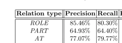
With the supervised SNoW learner, we get a 77.37% accuracy, and the class-specific performance is summarized in Table 6.
Table 5.Performance of supervised SVM learner (full)
Relation type Precision Recall F-measure ROLE 86.27% 85.96% 86.11% PART 75.90% 58.36% 65.89% AT 78.87% 88.65% 83.46% NEAR 83.96% 3.57% 8.41%
Table 6.Performance of supervised SNoW learner (full)
Relation type Precision Recall F-measure ROLE 85.46% 80.30% 82.19% PART 64.93% 64.40% 64.50% AT 77.07% 79.77% 77.77% NEAR 28.94% 27.95% 24.56% SOC 79.69% 84.32% 81.21%
Table 7.Performance of supervised naive bayes learner (full)
Relation type Precision Recall F-measure ROLE 52.63% 97.56% 68.37%
PART 0% 0% 0%
AT 78.13% 35.83% 48.82%
NEAR 0% 0% 0%
SOC 0% 0% 0%
With the supervised Naive Bayes learner, we get a 56.10% accuracy, and the class-specific performance is summarized in Table 7.
If we compare the performance presented in this subsection with those of the corresponding transductive learners in the previous subsection, we observe the following pattern:
NB<SGT<SNoW-SGT<SNoW<SVM-SGT<SVM
With regard to the purpose of this study, again, it is most important to no-tice that the induction-aided transductive learners significantly outperform the “pure” transductive learner. On the other hand, it is reasonable to expect that with improvement of the fundamental algorithm (e.g., spectral partioning), the transductive learners (with or without induced similarity measures) may out-perform the best inductive learners.
6
Conclusions and Future Work
This paper approaches the relation classification problem with improved trans-ductive learning. Specifically, we learned the following:
– Application of transductive learning on NLP problems, including informa-tion extracinforma-tion, has been under-explored. This paper makes the attempt to show that binary relations hidden in natural language text can be effectively classified by using transductive learning.
– Further more, the general idea of inducing similarity functions for trans-ductive learning are potentially applicable to other classification problems, since it doesn’t have any specific characteristics tied to the current relation classification problem.
In the future, we are interested in pursuing the following directions:
– The current work only deals with binary relations. The algorithms presented should be generalized so that they can work on higher-order relations.
– In this study, we only used a randomly selected portion of the labeled data available as the seed labeled set for inducing similarity functions. It is con-ceivable that if we anchor the seed data points more intelligently (e.g., using clustering or in other unsupervised fashion), better classification performance of the modified transductive learner can be expected.
– This chapter presents one particular way of inducing the similarity function for transductive learning, which is simple yet effective. However, it may be worth the effort to investigate other alternatives.
– In the machine learning community, how to exploit unlabeled data remains largely an open question. In the long run, it would be very interesting and useful to investigate, both theoretically and empirically, the tradeoff between induction with unlabeled data vs. transduction (including “induction-aided” transduction discussed in this paper).
References
1. Agichtein, E., Gravano, L.: Snowball: Extracting relations from large plain-text collections. In: Proceedings of the Fifth ACM International Conference on Digital Libraries. (2000)
2. Brin, S.: Extracting patterns and relations from the world wide web. In: WebDB Workshop at 6th International Conference on Extending Database Technology, EDBT’98. (1998)
3. Zelenko, D., Aone, C., Richardella, A.: Kernel methods for relation extraction. J. Mach. Learn. Res.3(2003) 1083–1106
4. Zhang, Z.: Weakly-supervised relation classification for information extraction. In: Proceedings of the 13th International Conference on Information and Knowledge Management CIKM 2004, Washington DC (2004)
5. Rosario, B., Hearst, M.: Classifying semantic relations in bioscience text. In: Proceedings of the 42nd Annual Meeting of the Association for Computational Linguistics. (2004)
6. Abney, S.: Understanding the Yarowsky algorithm. Computational Linguistics30 (2004)
7. Vapnik, V.N.: Statistical learning theory. John Wiley, NY (1998)
8. Joachims, T.: Transductive inference for text classification using support vector machines. In Bratko, I., Dzeroski, S., eds.: Proceedings of ICML-99, 16th Interna-tional Conference on Machine Learning, Bled, SL, Morgan Kaufmann Publishers, San Francisco, US (1999) 200–209
10. Blum, A., Chawla, S.: Learning from labeled and unlabeled data using graph mincuts. In: ICML ’01: Proceedings of the Eighteenth International Conference on Machine Learning, San Francisco, CA, USA, Morgan Kaufmann Publishers Inc. (2001) 19–26
11. Blum, A., Lafferty, J., Rwebangira, M.R., Reddy, R.: Semi-supervised learning using randomized mincuts. In: ICML ’04: Twenty-first international conference on Machine learning, New York, NY, USA, ACM Press (2004)
12. Kleinberg, J., Tardos, E.: Approximation algorithms for classification problems with pairwise relationships: metric labeling and Markov random fields. In: Pro-ceedings of the 40th Annual Symposium on Foundations of Computer Science. (1999) 14–23
13. Joachims, T.: Transductive learning via spectral graph partitioning. In: Proceed-ings of The Twentieth International Conference on Machine Learning (ICML). (2003)
14. Charniak, E.: A maximum-entropy-inspired parser. Technical Report CS-99-12, Computer Scicence Department, Brown University (1999)
15. Buchholz, S.: The chunklink script. (2000) Software available at
http://ilk.uvt.nl/~sabine/chunklink/.
16. Joachims, T.: Making large-scale support vector machine learning practical. In: Advances in kernel methods: support vector learning. MIT Press, Cambridge, MA, USA (1999) 169–184
17. Carlson, A., Cumby, C., Rosen, J., Roth, D.: The SNoW learning architec-ture. Technical Report UIUCDCS-R-99-2101, UIUC Computer Science Depart-ment (1999)