Feedback communication using orthogonal signals

FEEDBACK COMMUNICATION USING ORTHOGONAL SIGNALS

Thesis by

Stephen Stuart Lavenberg

In Partial Fulfillment of the Requirements

For the Degree of Doctor of Philosophy

California Institute of Technology Pasadena, California

1968

ii ACKNCWLEDGMENT

I greatly benefited from the guidance and advice of my research advisor, Dr. T. L. Grettenberg, and from several useful discussions with Mr. S. Farber, a fellow student. My studies were conducted under a National Science Foundation Graduate Fellowship and a National

Science Foundation Graduate Traineeship, and I am grateful for the financial assistance they have provided. I wish to thank my wife, whose constant encouragement and good cheer provided great impetus for

i i i ABSTRACT

This research is concerned with block coding for a feedback communication system in which the forward and feedback channels are independently disturbed by additive white Gaussian noise and average power constrained. Two coding schemes are proposed in which the messages to be coded for transmission over the forward channel are realized as a set of orthogonal waveforms. A finite number of forward and feedback transmissions (iterations) per message is made. Infor-mation received over the feedback channel is used to modify the

wave-form transmitted on successive forward iterations in such a way that the expected value of forward signal energy is zero on all iterations after the first. Similarly, information is sent over the feedback

Chapter I. II. III. IV.

v.

TABLE OF CONTENTS

INTRODUCTION ...••. · ..••••.•.•..•.•....•...•. FEEDBACK CODING SCHEME 1 . . . . 2 .1.

2.2. 2 .3.

Preliminaries ..•... Description of Scheme 1 . . . ... . . . Analysis of Scheme 1 . . . . FEEDBACK CODING SCHEME 2

3.1.

3

.2.

3.3.

'

3

.4.

Preliminaries ...•...•... Description of Scheme 2 ••••••••••••••••• Analysis of Scheme 2 . . . ... . . . . Peak Power ...•... PERFORMANCE OF THE CODI:r.G SCHEMES ... .

4.1.

The Channel Reliability Function .•...

4.2.

Comparison of Coding Schemes ...•...•.

CONCLUSIONS APPENDICES

A. Weak Converse for a Feedback Communication

l 5 5 6

8

20 20 20 21

32

36 36 36

43

System . . . • . . . . • . . . • . . . • . . 45 B. A Lower Bound to the Probability of Error

l

I. INTRODUCTION

This research is concerned with block coding for a communication

system consisting of a forward and a feedback channel. A block coding

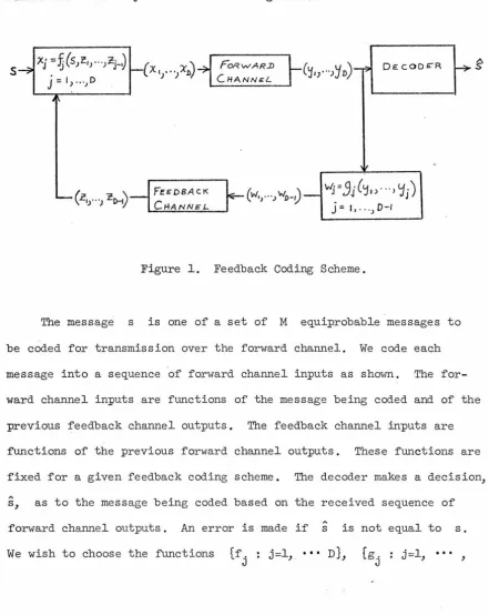
scheme for such a system is shovm in Figure l.

s

Xj ::t(s>~,,

...

>~j-~

j=l,

...

)D

FoR.vvAR.D C HANNt<L

De:cooE"R

Vlj=,9j(<ju···1<jj)

[image:5.554.55.497.156.711.2]

j

=

1,. .. ,D-I

Figure l. Feedback Coding Scheme.

The message s is one of a set of M equiprobable messages to

be coded for transmission over the forward channel. We code each

message into a sequence of forward channel inputs as shovm. The

for-ward channel inputs are functions of the message being coded and of the

previous feedback channel outputs. The feedback channel inputs are

fUnctions of the previous forward channel outputs, These functions are

fixed for a given feedback coding scheme. The decoder makes a decision,

"

s, as to the message being coded based on the received sequence of

"

forward channel outputs. An error is made if s is not equal to s.

D-l}, and the decoder so as to achieve reliable transmission of

infor-mation over the forward channel.

Feedback coding schemes have been analyzed under a variety of

assumptions regarding the forward and feedback channels [l-6]. These

schemes achieve a lower probability of error than that attainable

with-out feedback. The presence of the feedback channel does not, however,

increase the capacity of the forward channel. This result holds for a

wide class of feedback communication systems (see Appendix A).

In the remainder of this paper, we consider a feedback

communica-tion system in which the forward and feedback channels are independently

disturbed by additive white Gaussian noise and average power constrained.

While feedback coding does not increase the maximum rate at which

reliable information may be sent over the forward channel of this

system, it can improve error performance. If the feedback channel is

noiseless, Schalkwijk [2, 3], Kailath [2], Omura [4], and Butman [5]

have devised schemes in which the probability of error in transmitting

information over the forward channel is lower than the minimum

proba-bility of error attainable without feedback. This result holds at all

rates up to the forward channel capacity. These schemes use scalar

signals, that is each message is realized as a point on the real line.

The forward channel inputs are linear combinations of the scalar message

point being coded and the previous feedback channel outputs. The feed

-back channel inputs are linear combinations of the previous forward

channel outputs. Decoding is accomplished by taking an appropriate

linear combination of the forward channel outputs. Then, denoting this

3

representing the message being coded. In particular, the maximum

likelihood decoder may be implemented in this way. (Reference 5

con-tains the complete formulation of this linear coding scheme.)

Note that

a

is of the form

where n is a Gaussian random variable with mean zero and variance

2

a , and 8 is the message point being coded. If the message points

n

are equispaced about the origin, the probability of error, _{p '}

e for

this linear coding scheme is

p

e

where T is the time to transmit a message,

information rate of the forward channel, and

R _

ln

M

-

T

is the

y is the output signal

to noise ratio.

0

e

2

(y

=

- -2 ' where

cre

is the variance of the set of

a

n

equiprobable message points.) Clearly, as T becomes large, it is

necessary that y increase exponentially with time in order to

attain a vanishingly small probability of error for any non-zero rate R.

The above expression for the probability of error for a linear

coding scheme is also valid in the presence of feedback channel noise.

In this case y may be upper bounded by the sum ·or the ratio of

for-ward signal energy to forfor-ward channel noise and the ratio of feedback

result obtained by Elias

[

8

].

An alternate derivation of this bound,

which makes use of Butman's matrix formulation of the linear coding

scheme

[5],

is due to Farber

[9].)

Thus, with the average power

con-strained in both the forward and feedback channels, y can increase

no faster than linearly with time, and reliable transmission cannot be

maintained over the forward channel at non-zero rates. Equivalently,

for a finite amount of power in the forward direction, an infinite

amount of feedback power is required to maintain any non-zero rate, R,

and achieve a zero probability of error. This is a severe limitation

of linear coding schemes.

Kramer

[6]

has recently analyzed a feedback coding scheme in which

each message is realized as one of a set of orthogonal waveforms.

Information received over the feedback channel is used to modify the

waveform transmitted on successive forward iterations in such a way

that the expected value of forward signal energy is zero on all

itera-tions after the first. His scheme also achieves a lower probability

of error than the best one-way coding scheme at all rates up to the

forward channel capacity. However, even in the presence of feedback

noise, only a finite amount of feedback power is required to achieve

this improved performance. Thus, this scheme is of particular interest.

In

Chapters +I and III of this paper, feedback coding schemes are

introduced which further reduce the amount of feedback power required.

This is accomplished by sending information over the feedback channel

in such a way· that the expected value of feedback- signal energy is also

zero on all iterations after the first. Chapter IV contains a dis-' ""'

5

II. FEEDBACK CODIJ>G SCHEME 1.

2.1. Preliminaries.

The forward and feedback channels are the vector channel equiva

-lents of the time continuous additive white Gaussian noise channel .

(Chapter

4

of Referencell contains a discussion of the equivalence of

the vector and time continuous channel models.) Both channels are

assumed to have no bandwidth constraints, and the forward and feedback

noises are assumed to be statistically independent. Every T seconds

we wish to code and transmit over the forward channel one of M

equiprobable messages from the message set

' M}

Let

e

=

te.

₁ i=l, • • • , M}

be a set of orthogonal M dimensional vectors representing M

orthogonal waveforms over a time interval 'f with \\eill2

=

E. Let

i--1 J • • • , M}

be a similar set with \\¢i\\2 = E'. We associate each message s. 1

,J'

with a vector e. in

e

1 Let xk denote the M dimensional

in

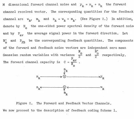
M dimensional forward channel noise and yk

=

xk + ~ the forward

channel received vector. The corresponding quantities for the feedback

channel are wk' and (See Figure 2.) In addition,

denote by N

0 the one-sided power spectral density of the forward noise

and by p

av the average signal power in the forward direction. Let

N~ and PFB be the corresponding feedback quantities. The components

of the forward and feedback noise vectors are independent zero mean

N

N'

0 0

~ and ~ respectively. Gaussian random variables with variance

p

The forward channel capacity is

xk

zk

C -~ _{- N} 0 nk

J-©

©

t ~ yk wk

Figure 2. The Forward and Feedback Vector Channels.

We now proceed to the description of feedback coding Scheme 1.

2.2. Description of Scheme 1.

Assume s £ ~ is the message to be coded for forward transmission

and

e

£ 8 is the M dimensional vector associated with s. We make

N forward transmissions and N-1 feedback transmissions, each of time

duration 1, as follows:

nl J,

xl

e

©

1

=

e

+ _nl

zl

¢1

+ ml @ wl =

¢1

1'

[image:10.549.50.487.60.447.2]

7

n2

*

l

*

x2

=

e

-

e

l

~@ Y2

e

-

e

l

+ n2

,...

zk

=

¢k - ¢k-l +

~"c--@----wk

=

¢k - ¢k-l

I

~

¢

k

*

where and

ek

are determined as follows:

Let

k

A.k = Y1 +

l:

(yj +

e.

i)

J

-j=2

over

and if ek = et then ¢k = ¢t•

Let

e.

E

e

J

(¢*

=

0) 0

¢

*k

Then is that member of which maximizes

*

and if ¢ _{k =} ¢ _t then Finally, if 9N

=

over

-lC·

ek = et.

¢.

E p

J

et the receiver decides st was the message

coded. An error is made if eN

f

e. Note that the total time T to transmit s is

T

=

NT

2.3. Analysis of Scheme l.

We wish to determine the probability of error, PN(e), the

average forward power and the average feedback power for this scheme.

In particular we wish to determine the behavior of these quantities as

we let 'f .... 00 _{while the rate of transmission, R =}

:4,

_{and N are}

held constant. Bounds on these quantities wil l be obtained in terms

9

Let

f(x) 1

-2

y

JM

-

1

2

_{dy dcx}

We define

Pefb

=

~

;J

where S'

E

_T

'

and

f(~)

where

s

= E -T

The properties of f(x) are well known and the reader unfamiliar with them should consult Chapter

5

of Reference ll. In particular, f(x) is monotone decreasing in x.

In the previous section we defined vector quantities A.k and 13k

*

which were used in determining ek and ¢k. If s is the message

being coded, then

*

and if e. e.

J J

k

Ak = k9 +

L

for j 1,

...

k

A.k k9 +

l:

n. _J j=l

In this case the probability that

*

(e. - e.)

J J

'

k-1 it follows that

Similarly,

*

"

and if ¢k-l

=

¢k-l then

*

"

In this case the probability that ¢k

f

¢k is simply Pefb" Hence,

is the probability that ek

f

e given that

••• , k-l and Pefb is the probability that

*

e.

=

e. for

J J

*

"

ek

f

ek given

*

ek-l = 9k-l" In what follows let £ ( ) be an operator denoting

statistical expectation and P( ) denote the probability of the

event in parentheses.

I.et

Then

where

=

P(ek

f

e./s. _{J.. J..} is being coded)

11

An upper bound to Pk(e) may be derived as follows:

*

,...

Pk(e/s. )= Pk(e/s. ,e. = 8.

l. l. J J

*

,...

for j=l,•••,k-1) P(8. = e. J J for

*

,...

j=l,···,k-l/s

1. ) + Pk(e/sl. .,eJ .

f

e. J for some j)

. k-1

*

,...

for some j/s.) = P k(l-P fb) + Pk(e/s.,e. -f e. for

l. e e l . J J

k-1

some j)(l-(1-Pefb) ) (2.1)

since

k-1

*

IT

*

,...

*

P(e. = e. j=l,···,k-1/s.) = P(e.

=

e./s., e~

J J l. . 1 J J l. 'V

J=

Noting that

it follows from (2.1) that

k-1

=IT

P(e~

=

. 1 J

J=

(1-P )k-1 efb

*

e./s., e. ₁ J l.

J-e

t-1 • • • J. -1)

t - ' '

e.

_J-

1)

It also follows directly from (2.1) that

We now obtain bounds on P where

. av

N

Pav =

~,.

L

dllxk\12)

k=l

=

~T

(

E

+

~

e(\\xk\\

2

))

For k ~ 2,

*

*

A

If ek-l

f

ei then either ek-l

f

ek-l or

ek ₁

!

e./s.)

- l. l.

Therefore,

where

(2 .3)

(2

.4)

13

* ...

and by induction, noting that P(e₁

f

e₁)

=

Pefb' we have

(2.6)

It follows from (2.2), (2.4), (2.5) and (2.6) that

Hence,

(2. 7)

We now bound PFB where

N-l

PFB =

~'f

L

dllwkli2)

k=l

(

N-l )

=

~'

E' +

~2'

<hll2)

(2.8)

,.

Now if ek

I

ek-l then either ek

I

ei or ek-l

I

ei. It

follows from this that

,.

P(ek

I

ek_₁/si) s P(ek

I

ei/si) + P(8k-l

I

ei/si)

Therefore,

It follows from

(2.2), (2.8)

and

(2.9)

that

E'

- s

PFB

NT (

N-l

,;;

~~

i + 2

~

2

( Pek + (k-i)

Finally, noting that Pek s Pek-l we obtain

SI SI ( 2

N

s

PFB

s

N

l

+

2(N-2)

Pefb +

(2.9)

(k-2)

pefb))

(2.10)

We now wish to determine the asymptotic behavior of this scheme

for large 'T. It follows from the properties of the function f(x)

that

for

for

k > l

S' S

1

5

and

p -+ 0

el as T -+ "" for 0

lnM

s

~ -- <

-T N

0

Therefore, for

S'

s

and 0 ~ R lnM

s

- ~

NT <

-N' N NN 0

0 0

we have

p -+ -

s

as T -+ ""

av N (2.ll )

PFB -+ -S' as T -+ ""

N

(

2

.1

2)

To observe the asymptotic behavior of the probability of error we examine the behavior of the channel reliability function, E (R), where

From Eq.(2.2) we have that

Let us now consider the following two cases:

A) S

NT

'

0

s

r'N

0

In this case

Therefore,

and

p

er

PN(e) $ N P

er

and

E(R) ~ lim

T-+C:O

(-

~

_NT tn P ) _er +

r

(

-

1

per)

=N

l

,.

__

im -rT tn

lim T-+c:o

Making use of the asymptotic expression for

E(R) ~ ­r N

s

tnM

2N - rT

0

(

-

;T

tnN)

P we have

er

We now require that

R

<~ _{NN .} Then using (2.ll) and (2.12) the

0 above result may be rewritten as:

If

then

p

av

r

-N 0

l7

0 ~ R . av av

(

rP P )

~min ~, No

E(R) ~

(2.l4)

. av

( rP

:rrun ~'

B) r ;?:: N (r need not be an integer)

In this case

so that

and

E(R) ;?:: _{( -}

~

-Ln p ) +

NT eN

lim

T-+CO

=

lim T-4D

(-

~

_NT

{,

n

P _eN )

s

_{R 0 ~ R}

s

2N - ~ 4N

0 0

=

(~

-JRr

s

s

4N

~ R < -_N

In additio~ from (2.3) we have that

Therefore,

E(R) s lim _(-

~

_{tn P}

)+

lim ( N l - ~-~ tn(l- -P ) )

NT eN NT efb

'!"->CO 1"->eo

lim

(-

l _peN

l

::: - t n

T_,co NT

provided that Pefb _, 0 as T _, ""'· This will be true as long as

lnM Si

-,.-

<NT

.

0

Finally, if we require that R < NN

s

, then using (2.ll) and (2.l2) 0

the above results may be rewritten as:

If

then

E(R) ==

NP av

W- -

R

0

r ;;:: N

0 s R s _mm . (NP_~, av Pav) _N

0 0

(NP p

l

. av av

min

rm- ,

W-

s R 0 -o I

p

<~ N

0

(2.l5)

19

The upper bound to E(R) obtained here from (2.3) also applies

to the case 1 ~ r < N. However, in that case the upper and lower

bounds no longer coincide. A more exact analysis is required to

obtain the true value of E(R) in that case. In the following

chapter a feedback coding scheme is introduced for which an exact

expression for the channel reliability function is obtained.

A discussion of the performance of these schemes is postponed

III. FEEDBACK CODING SCHEME 2

3.l. Preliminaries.

Section 2.l of Chapter II applies verbatim to Scheme 2. In

addition, quantities defined in Chapter II are not redefined in this

Chapter unless their meanings have changed. The feedback coding

scheme introduced here permits an exact analysis of the channel relia

-bility function. In addition, a simple modification of this scheme is

considered and its effect on peak power is discussed.

We now proceed to the description of feedback coding Scheme 2.

3.2. Description of Scheme 2.

Assume s c: ~ is the message to be coded for forward trans-mission and 9 c: 8 is the M dimensional vector associated with s. We make N forward transmissions and only one feedback transmission,

21

In this scheme we let

N

f..N = Y1 +

L

(yk + e1) • k=2

*

*

eN is then determined as in Scheme 1. e

1,

¢

1,

¢

1 and e1 are the

same as in Scheme 1.

3.3.

Analysis of Scheme 2.

We first obtain exact expressions for P and P

av FB' N

Pav -

;T

L

E(llxkll

2)

k=l

For k ~ 2,

*

2EP(e₁

r

e./s.)

where

Pefb' To do this we write

Therefore,

and

1

23

Also

Therefore,

(3.2)

We now consider PN(e), the probability of error, for this

scheme. Note that when s is the message being coded,

The probability of error therefore depends on the values of

e

1 and

*

e

₁. The following is a table of the possible events associated with

these values.

Event

A

B

c

D

It is assumed that s. is the message being coded.

1

e.

J

e

.

J

e.

₁

e

.

1 jfi jfi

e.

J

e

₁

.

j,h

e.

J

e.i

ifi, j

k=l N

L

nk + (2N-l)9₁ .-(N-l)8_J .

k=l N

2=

~+

k=l N

2=

~ +

E

e.

j.fi

J

e.

l.

These events are disjoint and we may write

A

2=

k=l

n. + e. + (N-l)e.

.K l. J

PN(e/si) = P(eN.tei/si,A)P(A/si) + P(8N

t

ei/si,B)P(B/si)

A A

+ P(eN

t

ei/si,C)P(C/si) + P(eN

t

8i/si,D)P(D/si)

A

+ P(eN _J_ e./s.,E)P(E/s.)

F i i l.

We wish to consider the terms which make up this sum.

~ P((A.._, _{. ".N} 8.) _J ~ (A.N'

e.

_l. )/s .,D) _l.

(3 .3)

We now substitute the value of A.N corresponding to event D in the above expression. When we do this we can condition the probability

o~y on the relationship

implied by event D. Therefore,

=

p

(

t

k=l

N

(nk, ej) + (N-1) E

~

L

(nk' ei) k=l

25

k=2

N

where

L

(nk, e j) and

k=2

are independent identically

dis-tributed Gaussian random variables.

It therefore follows that

(3.4)

A similar argument shows that

The conditional probabilities of events D and E are

and

P(E/s.)

J.

Now

P(eN-!= e./s.,B) _{J. i}

=

1 - P((A.N,e.) _J. > (A.N,e) _r

~

l -

P

(

~

1

(nk,e

1)

+ (2N-l) E >

~

(3.7)

for all r-/= i/s.,B)

. J.

N

(nk, ej )- (N-1) E,

L

(nk, er)

£or all r

f

i,j/(n~ei)

+

E

>

(n

1

,er)

£or

all

r

f

i)

::;; l - for all r

f

i/(n₁,ei)

+ E >

(n

₁

,er) for all r

f

i)

"

=

P(eN -f e./s.,A) 1. 1.

and

If

then

The conditional probabilities of events

A

and

B

are

lnM

s'

Q : : ; ; <

-T N'

0

p -+ 0

27

and for large T

In this case

"

0 ~ P(eN

f

ei/si,B) P(B/si) ~ P(eN

f

ei/si,A) P(A/si) (3. 8)

Finally,

(3. 9)

It follows from

(

3

.

3)

-

(3.9)

that

(3.lO)

where we have assumed T is large and 0 ~ -tnM < -S' to obtain the

T N'

0

upper bound.

Suppose now that

8 I S

N1

=

r N""" for r ~ l (r need not be an integer)

This implies

If, in addition, we require that

then

and from (3.l)

0

~

R

<~

NNO

p --+ 0 el

p --+ 0 efb

s

p --+

-av N

as

as

as

Equation (3.lO) is valid with

reliability function

E(R) = lim

[-T-+eo

where

T --+ co

pefb = p _er

~ln

NT PN(e))

(3.ll)

29

El(R) = l:i.m [-

~

ln p )

,._,co

NT eN

and

Now, using (3.2), (3.ll) and the asymptotic expressions for Pel'

Per and PeN' the above results may be written as:

If

then

where

NP

av

~-R

0

r :e: l

0 ~ R ~ . av ~

(

NP P )

min

W--,

N

0 0

. av av

(

NP p )

~in~' No ~ R

p <~

N 0

(3.l2)

(3 . l3a)

and

(r+l)P

_ _ _ a_v - 2R

2N 0

p

0 s R s av

4N

0

(r+2 )P av 2N

0

~

av s . av

P (rP

4N

Rsmmw-,

::v)

(r+l)P av N

0

0

2~

(l+/;) + 2R

0

0 0

( rP

. av

min~,

p

< av N

0

(3 .l3c)

These eQuations completely describe the behavior of E(R) for this

scheme. If N s r or N ~ r + l they can be simplified as follows:

Clearly

so that

as in Scheme l.

rP av

~-R

0

. av av

(

rP P )

0 s R s min ~ , N

0

. av (

rP

min ~'

for N s r

p

< ~

N

0

Therefore,

(r+l)P

_____ a_v __ R

2N

0

31

. av av

(

(r+l)P P )

0 :-s:: R :-s:: min 4No ' No

. av av

(

(r+l)P P )

min 4No ' No :-s:: R

for N ~ r + l

p

<

2:.!

N

0

Note that E

2(R) is independent of N. Hence, E(R) cannot be

in-creased by further increasing N, for N ~ r + l.

Before concluding this section it is of interest to consider the

p p

performance of this coding scheme when

N"E('

< N av We show that in

0 0

this case reliable transmission of information over the forward

channel is not possible at all rates up to the forward channel

capacity.

To see this, note that if

then

lnM S'

~ ~

N'

so that Pefb ~ 1 as ~ ~ ~

It then follows from (3.1) that

Pav -

~

(2N-l)

as T - oo

and from (3.10) that

for all rates R such that

av

p )

p

<~

N

0

Reliable transmission cannot be maintained for this range of rates.

3

.4.

Peak Power.

We define peak power for the feedback coding scheme as the

maximum average -power over any transmission interval T. let PPK

denote the peak power in the forward direction and PPK denote the

peak power in the feedback direction. The peak -power in the forward

direction is the maximum value of

llxkl!2

k

1,

• • • ' N T

If

e1

*

f:.

e

then

llxkll2

28 k 2, • • • ' N

= =

33

Therefore,

The peak power in the feedback direction is

Hence, from (3.2)

N

For the remainder of this section we assume that

and

Then from (3.ll)

S'

N'

0

s

rN

0

0

~R <~

NNO

PPK

- - -+ 2N

p av

as

r ~ l

(3.14)

Thus the ratio of peak power to average power increases with N,

transmissions is limited.

Suppose now we modif'y feedback coding Scheme 2 by letting

k

=

2, • • • , N

where g is a fixed positive gain constant. For this scheme we let

N

A.N = Y1 +

L

(yk + gel)

k=2

to determine 9N. Note that

p av

s

+

-N as T

-+ co

independent of the choice of g. Now, however,

Since,

PPK 2 .

p---

=

max(2g N,N)

av

we assume that only the constraint on the forward peak to average

(3 .15)

power ratio is critical. We wish to determine tlJ.e channel reliability

If then where p av 2N 0

E₁(R) =

v~:v

PFB _{rP av}

N'

=

-w---0 0

( (N-l)g+l) N

( (N-l)g+l) 2 N

2 - R

-JR

r

35

r ~ l

<R<min(

2

Pav

J

( (N-l)g+l) p

0 av

N

4N

J

No

j

0

. ( ( (N-l)g+l)2 p _{av p ) p}

_ £ sR< _ £

min N

4N

_{J N}

N

0 0 0

and E

2(R) is again given by (3.l3c) and is independent of N and g. E

1(R) can be increased by increasing either Nor g. However, if we fix the forward peak to average power ratio (see (3.15)), it can be shown that

E1(R)

increases with decreasing g (for g ~ J2/2).

Therefore, it is reasonable to choose g

=

l as in feedback coding

Scheme 2, and increase ance. E₁ (R) is

g

=

[2/2

and

N

in fact PPK

= p

av

N in order to obtain maximized, for fixed

improved error

perform-p PK

IV. PERFORMAl'fCE OF THE CODING SCHEMES

4.1.

The Channel Reliability Function.

In Chapters II and III of this paper we analyzed two block coding schemes for a feedback communication system in which the forward and

feedback channels are disturbed by independent additive white

Gaussian noise and average power constrained. In particular, we focused our attention on the behavior of the channel reliability

function, E(R), for these schemes. (See Equations (2.13)-(2.16),

(3.12) and (3.13).) This function is of particular interest since for large coding delay (time to transmit a message) T, the probability

of error is given by

PN(e) ""'exp(-E(R)T)

and E(R) can be used to compare the performance of different coding schemes.

4.2. Comparison of Coding Schemes.

The channel reliability functions for the feedback coding schemes can be compared with the optimum reliability function attainable if

the feedback channel were not available. Denoting this optimum

p

av 2N - R

0

37

EI (R)

(4.l)

p p

av ~ R < av

'l:j:N N

0 0

It is well known that signals orthogonal over the time interval T

attain this performance. Note that for both feedback coding schemes, E(R) >EI (R) at all rates R up to the forward channel capacity,

p

C - _!!:".'!_

- N '

0

provided only that the feedback channel capacity be greater than· the

T,

forward channel

p

and R <

..E-N ₀ '

capacity. Hence, for the same values of the probability of error, for the feedback schemes is less than the probability of error, P'(e) ::::.. exp(-E' (R)T), for the best one-way scheme.

p av'

As T becomes arbitrarily large for these schemes, so does the number of dimensions per second used in coding, or equivalently, so does the bandwidth used [ll]. In many practical systems we may be restricted to a given large but finite time-bandwidth product, or equivalently, to a given large but finite number of dimensions. It is interesting to compare the one-way and feedback schemes for the same

p values of Pav' N

0, R

<

N av , and the same large but finite number

0

of dimensions D. Letting M' denote the number of messages and T' the coding delay for the one-way orthogonal scheme, we have

and

D = M'

Using (4.1), it then follows that

p ~

4;v

0

P'(e) ""'exp(-E'(R)T') =

(4.2)

p p

av ~ R < ~

4N

N

0 0

Letting M denote the number of messages, T the coding delay, and

N the munber of forward transmissions for the feedback coding schemes,

we have

and

D

=

MN •

39

f

exp

{

_(NP

av _ l) ln

~1

p \

N:VJ

\ 2N R N

PN(e) ""' exp(-E(R)T)

=l

o

(4.

3)

\2 NP p

ex{(Jif-

l)

ln

~)min(~, N:v)~

R

p <~

N

Using (4.2) and

same p

av'

(4.3)

it can be shown that PN(e) < P'(e) for the

p

R < av and number of dimensions D which is

N ₀ '

assumed to be large.

0

We now discuss the relation of Schemes 1 and 2 to existing

feed-back coding schemes. In Chapter I we mentioned several existing

coding schemes for the particular feedback communication system we

have considered. It is worth repeating that in the presence of feed

-back noise the schemes of Schalkwijk [2,3], Kailath [2], Omura

[4],

and Butman [5] require an infinite amount of feedback power to maintain

any non-zero rate and achieve a zero probability of error. Hence, the

presence of feedback noise poses a severe limitation on the performance

of these schemes. The scheme considered by Kramer

[6

]

does not have

this limitation, however. Even in the presence of feedback noise, his

scheme requires only a finite amount of feedback power to achieve

im-·proved asymptotic performance over the best one-way scheme at all

rates up to the forward channel capacity. His is the first feedback

coding scheme.with this property. Kramer's sche~e uses ,N forward

transmissions and N-1 feedback transmissions and is similar to

If

then

E(R)

=

NP

av

~-R 0

r :?: N(N-1)

. av av

(

NP p )

0 ~ R ~ min ~ , No

. av av

(

NP p )

mm~, No ~ R

p <

....!E:!..

N

0

(4.4)

(4.5)

To obtain the same performance as in

(4.5)

for the same number, N,

of forward transmissions, Schemes 1 and 2 require only that

p

av r - -_N

0

r:?: N

(See Equations (2.15), (2.16), (3.12), and (3.13).) Of course the

condition

(4.4)

on the amount of feedback power required is only a

sufficient condition. As Kramer points out, it may in fact be

possible to obtain the s&me E(R) for a smaller value of the feedback

power.

With this in mind, a lower bound to the probability of error for

Kramer's scheme is obtained in Appendix B. (S~e _Equations (B.8) and

•

4l

where r is an integer greater than 1 and that N

=

r + 1, Let

EK(R) denote the channel reliability function for Kramer's scheme.

It follows from (B.9) that

(r+l)P av

- (r+l) R

p

0 s; R s; av

4N

0

=

(4.6)

(J

(r+l)P

)

2

No av - j(r+l)R

p p

av s; R < ..E_

4N

N

0 0

The channel reliability function, E(R), for Scheme 2 with N r + l

is given by (3.13c), which is repeated here for convenience.

(r+l)P p

av

- 2R 0 s; R s; av

2N

4N

0 0

(r+2 )P

15

P

(r

P

::v)

E(R) _2N av 2 __:::...

4N

av s; R s; min .

4N"" ,

av (3 .13c) N

0 0 0 0

(r+l)P

~

(rP

P

)

P

av . av av < av

N 2 N (l+Jr)+ 2Rmrn~, N s: R N

It follows from the above that E(R) > EK(R) for R > O. In particular, it can be shown that

E(R) ~ EK(R) + (r-l)R

and for r ~ 4

p

E(R) ~ EK(R) +

4

:v (r-l)

0

p av

O~R~Ij:N

0

p p

av~ R < ~

4N

N

0 0

Kramer uses equal amounts of energy on each feedback transmission rather than using all the available energy on the first transmission as in the forward channel. By sending information over the feedback channel in such a way that the expected value of feedback signal

energy is zero on all transmissions after the first, Schemes 1 and 2

achieve a reduction in the amount of feedback power required.

Finally, it should be mentioned that for N

=

2, Schemes l and 2

43

V. CONCLUSIONS

A feedback communication system in which the forward and feedback

channels are independently disturbed by additive white Gaussian noise

and average power constrained was considered. Feedback coding schemes

were presented which make efficient use of the feedback power available

to obtain improved error performance over existing coding schemes. The

behavior of the probability of error is particularly dramatic at rates

arbitrarily close to the forward channel capacity, since channel

reliability functions were obtained which remain positive at capacity.

The messages to be coded were realized with a set of signals (in

this case orthogonal signals) which allow reliable one-way transmission

of information over both the forward and feedback channels. The

ex-pected value of signal energy in both the forward and feedback channels

could then be made negligible on all iterations after the first. In

this way all the available signal energy per message could be used on

the first iteration, and the probability of error was decreased. This

approach can be applied under other assumptions regarding the forward

and feedback channels provided that signal sets exist which allow

reliable one-way transmission of information over these channels. If

the average power were the critical factor in determining the error

probability for the forward channel, improved error performance should

be obtainable in this way.

It should be pointed out that the coding schemes presented here,

while effective, are not optimum. Several modifications are possible.

Signal gain constants could be used. However, it was shown that peak

iterations per message as a means of improving error performance

rather than using gain constants. The decoder considered is optimum

only if the feedback channel is noiseless, and it could be modified.

It is, however, desirable that the decoder still be easy to implement

and analyze. The decision rule used on the feedback channel could

APPENDIX A

WEAK CONVERSE FOR A FEEDBACK COMMUNICATION SYSTEM

Consider the feedback coding scheme of Figure 1. If the forward

channel is discrete and memoryless and the feedback channel is

noiseless, Shannon

[

7

]

has shown that such a scheme cannot increase

the capacity of the forward channel. This result is now extended to

a system in which the forward and feedback channels are independent,

time discrete, amplitude continuous, and memoryless. In what follows

we assume that all random variables have bounded density functions and

finite variances so that all integrals exist.

Let p(y/x) be the conditional probability density describing

the forward channel, where the channel inputs x and outputs y are

points on the real line. Let / denote the set of M messages to be

coded for transmission over the forward channel and V denote the

space of forward channel output sequences (V is Euclidean D-space).

We assume the forward channel inputs are constrained so that

1

n

e:(h(xJ .)) ~ K

where E( ) is an operator denoting statistical expectation, h is

a real-valued fUnction, and K is a constant. I.et

I(./;v)

=

L

f

P(s) p(v/s) ln

P~(t))

dv

Jv

.

Let

CD CD

r(x;Y) ==

J

J

p(x)p(y/x) in

P~ci))

dy dx _co -CD

be the forward channel mutual information, and

C == Max _CD I(X;Y)

p(x) :

J

p(x)h(x)dx

~

K

be the forward channel capacity.

We now prove the following

Lemma.

r(J;v)

~

nc

Proof: Since the channels are independent and memoryless, the

channel output yj depends only on the channel input xj. Therefore,

Making use of this, Gallager has shown (see Appendix A of

Reference

4)

D

I(../;V)

~

L

Ij (X;Y) j==l

The mutual information, Ij(X;Y), is computed using the density,

pj(x), on the jth channel input for the given feedback coding scheme.

D

p'(x) =IT

L

pj(x) j=l

Let I'(X;Y) be the mutual information computed using this density

:function. Letting

co co

pj(y)

~

pj(x)p(y/x)dx and p'(y) =

f

p'(x)p(y/x)dx

_co -CO

we have

co co co

I' (X;Y) =

J

_{p' (y)ln p' (y) dy -}

J f

_{p' (x)p(y/x) ln}

p(~/x)

dy dx

-CO _co _co

D co D co co

= IT

L

f

P/Y)ln p'

CY)

dy - IT

L

f

J

p/x)p(y/x) ln

p(~/x)

dy dx

j=l -CO j=l -co -CO

D ( co

;:: IT

L

f

pj(y)ln p.ty)

. l J

J= -co

D

=

IT

L

Ij (X;Y) j=l

Hence

co co

dy -

J

J

pj (x)p(y/x)ln p(ylx)

r(..!;v) ~DI' (X;Y)

D oo

~

L

J

pj (x) h(x) dx

~

K j=l -<Xl

Therefore, p'(x) satisfies

CXl

J

p'(x) h(x) dx

~

K

and

I ' (X;Y) ~ C

The proof is complete.

Assuming the messages are equiprobable, we now have the

following.

Theorem (Weak Converse). If R =

D

lnM >

c,

the probability of error, P(e), for the feedback coding scheme is bounded away from zero.

Proof: The proof is standard (see Chapter

8

of Reference 10). Let

Then

H(..//v)

=

L

J

P(s/v)p(v) ln P(;/v) dv

..!

v

' ( J 1 1

H( ..

.//v)

~ P(e)ln

P(e)

+ (1-P(e))ln l-P(e) + P(e)ln(M-1)

messages,

I(J';V) 1nM - H

(..//v)

Application of the lerruna now yields the weak converse.

Hence, feedback coding cannot increase the capacity,

c,

of the forward channel. In particular, the above results apply to the

APPENDIX B

A LCMER BOUND TO THE PROBABILITY OF ERROR FOR

KRAMER'S SCHEME

The symbols to be used here have been previously defined in

Chapter II. The description of feedback coding Scheme l (see Section

2.2) applies to Kramer's coding scheme

[6]

with the following changes.

We transmit

k = l, • • • , N - l

over the feedback channel and let

k = l, • • • , N-l

*

*

~

to determine ¢k. Note that the probability that ¢k

f

¢k is simply

pefb' independent of the values of

¢:

~

It can be shovm for this scheme that

p

av

(N-l)S I

N

(See Chapter III of Reference

6.)

and t=l, ••• ' k-l.

(B.l)

(B. 2)

5l

We now obtain a lower bolilld to the prooability of error for this scheme. To do this we consider. the following table of events

(similar to that in Section

3.3)

associated with the possible values

*

of eN-l and 9N-l" It is assumed that s. l. is the message being

coded.

Event 9

N-°1 9

*

N-l "-N = "-N-1 + YN + 9_N-l

AN-l e. l. e. l. "-N-l + ~ + 9l. .

B _{ei ej j;fi A.N-1 + ~+} 29.

-

9.

N-l· l. _J

CN-l e. _J j;fi e_J . "-N-l + ~ + ei

DN-l e. _J j;fi e .{, .if i, j A.N-l + ~+ e. l.

-

e .i + ej

EN-l e. _J jfi e. l. A.N-l + ~+ e_J .

The method of analysis is similar to that of Section

3.3.

The events are disjoint so that

A A

PN(e/si) P(9Nf ei/si'~-l) P(~_

1

/si) + P(eN

f

_{9i/si,BN_1 )P(BN-l/si)} A

+ P(eN

f

ei/si,cN-l) P(CN-1/si) + P(eN

f

ei/si,DN-l)P(DN-l/si) A

+ P(eN

f

ei/si,EN-l) P(EN-l/si) (B.4)

P(eN

f

_{ei/si,DN_1 )}

=

P((AN,er) ~ (AN,ei) for some r

f

_{i/si,DN_1 )}

<~-1'

ei >)

;;:.: P( (nN'

e

j

>

~

<,,

e

i

>

)

l

=2

Similarly, it can be shown that

The conditional probabilities of events DN-l and EN-l are

and

Lower bounding the second term in (B.4) by zero, it follows from

tne above that

.... ....

PN(e/si) ~ P(9N

f

ei/si,~-l)P(AN-l/si) + P(9N

f

ei/si,CN-l)P(CN-l/si)

53

It is difficult to obtain an exact expression for the first two terms in (B.5). However, a simple lower bound to these terms follows from

noting that

= p (1-P )N-1

eN efb

Therefore,

for k = 1, ••• _{, N-1/s.)}

1

P (e) P

PN(e)

~

p (1-P )N-1 + N-1 efb (B.6)

eN efb 2

A similar lower bound to PN_₁(e) may be obtained. Substituting this

lower bound in (B.6), lower bounding PN_

2(e), and continuing in this way, the following lower bound to PN(e) is obtained.

(B .7)

Suppose now that

Then

O:SR<~

NN

0

Pek < Pel -> 0 as T -> oo for k > l

= p

r

e N-l

,and if N :S r + l then

It then follows fro~ (B.l) and (B.3) that

s

P .-. - as

av

N

Using (B.2) and (B.7), it follows from the above that If

r ;;::: l and N :S r + l

then

55

N (

Pe

N~ll

k-l (

p e

N2~liN-k

PN( e)

~

L

P ek l

-k=l

(B. 9)

REFERENCES

[l] E. R. Berlekamp, "Block Coding with Noiseless Feedback", Ph.D.

Dissertation, M.I.T., Department of Electrical Engineering,

September 1964.

[2] J. P. M. Schalkwijk and T. Kailath, "A Coding Scheme for Additive

Noise Channels with Feedback - Part I: No Bandwidth Constraint",

I.E.E.E. Transactions on Information Theory, IT-12, 172-182, April 1966.

[3] J. P. M. Schalkwijk, "A Coding Scheme for Additive Noise Channels

. with Feedback - Part II: Band-Limited Signals", I.E.E.E.

Trans-actions on Information Theory, IT-12, 183-189, Apri l 1966.

[4] J. K. Omura, "Signal Optimization for Channels with Feedback",

Report SEL-66-068, Stanford Electronics Labs., Stanford University,

August 1966.

[5] S. Butman, "Optimum Linear Coding for Additive Noise Systems Using

Information Feedback", Technical Report No. l, Communications Theory Lab., California Institute of Technology, May 1967.

[6] A. J. Kramer, "Analysis of Communication Schemes Using an

Intermittent Feedback Link", Report SEL-67-014, Stanford Electronics Labs., Stanford University, March 1967.

[7] C. E. Shannon, "The Zero-Error Capacity of a Noisy Channel",

I.R.E. Transactions on Information Theory, IT-2, 8-19, September

1956,

[8] P. Elias, "Networks of Gaussian Channels with Applications to

Feedback Systems", I.E .E .E. Transactions on Information Theory,

IT-13, 493-501, July 1967.

[9] S. M. Farber, Private Communication, 1968 (to be published).

[10] R. B. Ash, Information Theory, John Wiley and Sons, Inc., New York,

1965.