the Partition Function of the Ising Model
Thesis by
Ming-Shr Matt Lin
In Partial Fulfillment of the Requirements
for the Degree of
Doctor of Philosophy
California Institute of Technology
Pasadena, California
2009
c
2009
Ming-Shr Matt Lin
Acknowledgements
I would like to express my deep appreciation to Dr. Wilson. For without his support and
encour-agement, not to mention professional advice on my research, it would be impossible for me to go
through the whole process. I learned not only how to do research in a professional manner, but
also how he advised me in a patient and encouraging way. I would also like to thank Dr. Cross,
Dr. Preskill, and Dr. Wales for serving my examination committee. Their presence and guidance
during my defense will certainly increase my intellectual ability and provide me outlook for future
Abstract
The research work discussed in this thesis investigated the application of combinatorics and graph
theory in the analysis of the partition function of the Ising Model.
Chapter 1 gives a general introduction to the partition function of the Ising Model and the
Feynman Identity in the language of graph theory.
Chapter 2 describes and proves combinatorially the Feynman Identity in the special case when
there is only one vertex and multiple loops.
Chapter 3 digresses into the number of cycles in a directed graph, along with its application in
the special case to derive the analytical expression of the number of non-periodic cycles with positive
and negative signs.
Chapter 4 comes back to the general case of the Feynman Identity. The Feynman Identity is
applied to several special cases of the graph and a combinatorial identity is established for each case.
Contents
Acknowledgements iii
Abstract iv
1 Introduction 1
1.1 Review of the Ising Model and its partition function . . . 2
1.2 The partition function as a summation over graphs . . . 4
1.3 The partition function as a product over cycles: The Feynman Identity . . . 5
2 A Combinatorial Proof of a Special Case of the Feynman Identity 7 2.1 Introduction . . . 8
2.2 Proof of the identity . . . 9
2.3 Definition and properties of the sign function . . . 12
2.4 More on the sign function . . . 16
3 The Number of Non-periodic Reduced Cycles in a Directed Graph 20 3.1 Outline . . . 21
3.2 The number of non-periodic cycles . . . 21
3.3 The number of non-periodic cycles with specified occurrences of edges . . . 23
3.4 Non-periodic cycles with positive and negative signs in the special case . . . 25
4 Theorems Derived from the Feynman Identity 28 4.1 Introduction . . . 29
4.3 The first identity . . . 30
4.4 A combinatorial lemma . . . 33
4.5 The second identity . . . 36
4.6 Two more combinatorial lemmas . . . 38
4.7 The third identity . . . 41
4.8 The fourth identity . . . 44
4.9 The fifth recursion relation . . . 47
5 Conclusion 49 5.1 Conclusion . . . 50
A The Number of Pointed Cycles in the Case of Two Loops 51 A.1 Relation with Costa’s equation . . . 52
A.2 Derivation of the function for the number of pointed cyclesf(a, b) . . . 53
A.3 Comparison of the two functions . . . 54
A.4 Combinatorial interpretation offC(a, b) . . . 56
B Explicit Expression of the Feynman Identity When the Graph Is Connected 57 B.1 A special case of (4.3) when the graph is connected . . . 58
List of Figures
1.1 Ising Model . . . 2
2.1 Cotree with eight loops . . . 12
2.2 Illustrative graph for the change of revolution number . . . 14
2.3 Illustrative graph for calculation of change of angles . . . 15
2.4 Interlacing graph . . . 17
Chapter 1
1.1
Review of the Ising Model and its partition function
Graph theory has a natural application in the calculation of the partition function of the Ising model.
We will review the partition function of the two-dimensional planar Ising model and the key step in
the calculation, the Feynman Identity.
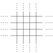
[image:9.595.277.371.276.369.2]The two-dimensional planar Ising model is defined on a square lattice Λ. Each siteiof Λ contains
Figure 1.1: Ising Model
a ‘particle’ with two possible states. A generic example of this model is as follows: Consider a solid
consisting ofN identical atoms arranged in the regular lattice defined above. Each atom has a net
electronic spinS~ and associated magnetic moment~µ=gµ0S. In the presence of an external applied~
magnetic fieldHzalong thezdirection, the HamiltonianHrepresenting the interaction of the atoms
with this field is then
H=−gµ0 N
X
j=1 ~
Sj·Hz. (1.1)
In addition, each atom is assumed to interact with neighboring atoms, but this is not just the
mag-netic dipole-dipole interaction. This interaction is in general too small to produce ferromagnetism.
The dominant interaction is usually the exchange interaction, a consequence of the Pauli exclusion
principle.
We will focus on the spin-1/2 situation and adapt the standard notation σi, instead of Si, to~
in the stateσi andσj respectively, is described by
Eij =
−Jσiσj if i, j are nearest neighbors(n.n.)
0 otherwise
(1.2)
whereJ is a parameter that describes the strength of the interaction and it tends to fall off rapidly
with increasing separation between two particles. Therefore, we consider only nearest neighbor
interaction. When J is greater than zero, the state of lower energy will be the one which favors
parallel spin orientation, i.e., one tends to produce ferromagnetism.
Suppose Λ has N2 sites, then there are 2N2
distinct configurations of the spins. CallS ={σ}
the set of all configurations of the system. The energyEσ of each configurationσ∈S is given by
Eσ=−J X n.n.∈σ
σiσj (1.3)
and the partition function is
Z =X σ∈S
e−βEσ (1.4)
Since we will formulate everything in the language of graph theory, let’s call the site vertex from
here on. We need two definitions before we state the main theorem.
Definition 1: An even graph G is a graph whose vertex have even number of degrees. A even
subgraphH of a graphK is a subgraph ofK andH is an even graph itself.
Definition 2: Given a graphG, define the single-variable polynomial related toGas
IG(u) =u|E(G)| (1.5)
1.2
The partition function as a summation over graphs
For completeness, we will include the relevant part in [6] to show that the partition function can be
written as a summation over even subgraphs.
Theorem 1.2.1 Let Abe the set of all even subgraphs ofΛ which containsN2 vertex, then
Z = 2N2(1−u2)−N(N−1) X G∈A
IG(u) (1.6)
whereu=tanh(K)andK=Jβ.
Proof.Let’s rewrite the partition function (1.4) as
Z = X σ1=±1
. . . X σN=±1
Y
n.n.
eKσiσj (1.7)
by substitution of (1.3) into (1.4), whereK=Jβ .
Sinceσiσj =±1, it follows that
eKσiσj =e±K= coshK±sinhK; (1.8)
therefore,
Y
n.n.
eKσiσj =Y
n.n.
coshK±sinhK
= coshBKY n.n.
(1±tanhK) = (1−u2)−2B Y
n.n.
(1 +uσiσj)
whereB = 2N(N−1) is the number of bonds in Λ. The factor (1−u2)−2Bcomes from 1−tanh2K=
cosh−2K; therefore, coshBK= (1−tanh2K)−2B.
To each pair (i, j) of nearest neighbors of Λ, there corresponds a termuσiσj and an edge. Since
product on the right-hand side is a polynomial in u of degree B, that is ,
Y
n.n.
(1 +uσiσj) = 1 + B
X
p=1 upX
n.n.
(σi1σi2). . .(σi2p−1σi2p). (1.9)
The second summation, i.e., the summation over n.n., is over all possible products of p pairs of
nearest neighbors of Λ where a pair is not to occur twice in the same product. Each pair (σi, σj)
is associated with an edge connecting verticesi andj; so each product of ppairs corresponds to a
graph withpedges. We see that the second summation is over all graphs with pedges. The graph
may have vertices of degree 0,1,2,3, or 4, in the situation of the planar lattice. The summations
over the spins, i.e.,σi’s, eliminates graphs containing any odd-degree vertex, becausePσi= 0 and
P
σ3
i = 0. The graphs left are those whose vertices all have even degrees. There is a factor of 2N
2
because each vertex of Λ contributes a factor of 2 from P
σ(even degree)i = 2, and the summations
include all theσi’s. Notice that in the proof, there is no need of planarity.
We will get rid of the constant in front of the summation and call the summation as the partition
function for simplicity.
The even graph we have here is not the physical diagram of the lattice itself. It is a
diagram-matic description of the proof above. For example, a vertex with degree 4 doesn’t mean that its
corresponding site has a spin that is parallel to its four neighbors, but that it has appeared four
times in the product.
1.3
The partition function as a product over cycles: The
Feynman Identity
In order to facilitate the calculation of the partition function and therefore predict the thermal
the following identity for a general graph embedded in a plane:
X
G∈A
IG(u) = Y [c]∈P
(1 +Jc(u)) (1.10)
where σ(c) is the sign of the cycle [c], defined in Chapter 2, P is the set of non-periodic reduced
cycles, defined in Chapter 3, andJc(u) =σ(c)Ic(u).
There have been a few articles on the Feynman identity [1][7] and its proof. The special case
when there is only one vertex first appeared in Sherman[2], but there is no rigorous proof of the
identity in that paper. In the special case, one can interpret the loops asgenerators and the cycles
asword, as will be shown in the next chapter. Therefore, we can assign combinatorial meanings to
both sides of the Feynman identity, and by double counting, the proof is done in a clear and short
Chapter 2
2.1
Introduction
The identity stated as Theorem 2.1.1 below was given by S. Sherman [2] as a special case of the
Feynman identity. This latter result has an involved geometric/topological proof. Sherman remarks
in [2] that “a strictly algebraic and non-geometric proof of [this theorem] would be in order... Such
an algebraic proof might shed light on the Ising problem in three dimensions.”
Let Fk be the free group onk generators x1, . . . , xk. Awordw=a1a2· · ·an inFk, where each
symbolai is one of the generatorsx1, . . . , xk or their inversesx−11, . . . , x− 1
k , is circularly-reduced, or
c-reduced, whenai+16=a−i1fori= 1,2, . . . , n−1 and alsoa16=a−1
n . It will be convenient to exclude
the identity inFk as a c-reduced word. From here on, all words will be c-reduced, so we may skip
the word when appropriate.
Letρbe the permutation of the c-reduced words that takes a1a2· · ·an to ana1a2· · ·an−1. The
images of powers of ρ on a word w are the rotations of w. A circular-word [w] is the set of all
rotations of a given c-reduced word, i.e. an orbit of the cyclic grouphρigenerated byρon the set of
c-reduced words inFk. We remark that the circular-words are in one-to-one correspondence with the
nontrivial conjugacy classes in Fk (every conjugacy class contains c-reduced words; two c-reduced
word are conjugates if and only if one is a rotation of the other). As we switch to the formulation of
a planar drawing of an oriented cotree in section 2.3, there is a natural correspondence between these
two languages: each generator corresponds to a loop in the special case, and each cycle corresponds
to a circular word, with two orientations considered as different.
Sherman defines asign σ(w)∈ {1,−1}for every c-reduced word w. The definition will depend
on an orientation of a planar drawing of a cotree (a graph with one vertex) withkloops labeled by
the generatorsxi. The definition of sign is geometric (involving paths and angles) and we must deal
with that. For the momment, we note only that the signs of a word and any of its rotations are the
same, so thatσis well-defined on circular-words.
The periodof a wordw (or circular-word [w]) is the least positive integer t so thatρt(w) = w.
A wordwor circular-word [w] of lengthnis said to benon-periodicwhen the period of wisn.
of non-periodic c-reduced circular-words [w] of length n=n1+· · ·+nk with σ(w) =ǫ, and which
contain a total ofni of the symbolsxi andx−i1 for eachi= 1,2, . . . , k.
Theorem 2.1.1 In the ring of formal power series ink(commuting)indeterminatesZ1, Z2, . . . , Zk, we have
Y
n1,···,nk≥0
(1 +Zn1
1 · · ·Z nk
k )
N(n1,···,nk;+)(1−Zn1
1 · · ·Z nk
k )
N(n1,···,nk;−)
= k
Y
j=1
(1 +Zj)2 (2.1)
where the product on the left is extended over all k-tuples(n1, . . . , nk)of nonnegative integers other
than(0,0, . . . ,0).
The proof of Theorem 2.1.1 is given in Section 2.2. In Section 2.3 we derive the algebraic
properties ofσwe use in our proof, and in Section 2.4 we observe a further property that allows us
to compute the sign of a c-reduced word combinatorially from the word and the cotree without any
reference to paths and angles as in the original definition.
TheWitt Identity [3] concerns the numbersM(n1, . . . , nk) of non-periodic circular-words in the
free semigroup generated byx1, . . . , xk, withnioccurrence ofxi for eachi= 1, . . . , k. Following the
notation of Theorem 2.1.1,
Y
n1,···,nk≥0
(1−Zn1
1 · · ·Zknk)
M(n1,···,nk)= 1
−Z1−Z2− · · · −Zk. (2.2)
It is in view of (2.2) that (2.1) is calledan Analogue of the Witt Identityin [2].
2.2
Proof of the identity
Properties ofσthat we require for the proof are
and
σ(ud) = (
−1)d−1(σ(u))d for every c-reduced wordu. (2.4)
For ǫ = ±1 and nonegative integers n1, . . . , nk, let W(n1, . . . , nk;ǫ) denote the number of
c-reduced words (not circular-words) that have sign ǫ and a total of ni occurrences of xi or x−i1, i= 1,2, . . . , k. We will need to know that givenn1, n2, . . . , nk, at leasttwoof which are positive, we
have
W(n1, n2, . . . , nk; +) =W(n1, n2, . . . , nk;−). (2.5)
Proofs of (2.3), (2.4), and (2.5) will be given in Section 2.3. Assuming these properties, the proof
of Theorem 2.1.1 is purely combinatorial.
We first give a relation between the numbers W(n1, n2, . . . , nk;±) andN(n1, n2, . . . , nk;±).
Lemma 2.2.1 Givenn1, n2, . . . , nk, not all zero, letgbe the greatest common divisor ofn1, n2, . . . , nk
and writen=n1+· · ·+nk. Then
W(n1, n2, . . . , nk; +) = X d|g, d odd
n dN(
n1 d ,
n2 d , . . . ,
nk
d ; +), (2.6)
and
W(n1, n2, . . . , nk;−) = X d|g, d even
n dN(
n1 d,
n2 d, . . . ,
nk d; +)
+ X
d|g n dN(
n1 d,
n2 d, . . . ,
nk
d ;−). (2.7)
Proof. The period of a c-reduced word with ni occurrences ofxi andx−i1 will be of the form n/d whereddividesg. Given a divisordofg, the c-reduced words withnioccurrences ofxiandx−i1, and periodn/d, may be obtained as follows: Start with a representativeuof a non-periodic c-reduced
circular-word [u] of lengthn/d withni/d occurrences ofxi andx−i1 and repeat itdtimes to get a c-reduced word w=ud. Associate to [u] the distinct rotations ofw, namely the firstn/d rotations
As dranges over divisors ofg, we obtain every c-reduced wordwwith ni occurrences ofxi and
x−i1 exactly once in this way. By (2.4), the sign σ(w) ofw =ud is (
−1)d−1(σ(u))d. Ifd is even, σ(w) =−1. If dis odd,σ(w) =σ(u). Therefore, every word [u] inN(n1
d , n2
d , . . . , nk
d ; +) withdodd
contributen/dwords inW(n1, n2, . . . , nk; +), and the rest contribute toW(n1, n2, . . . , nk;−).
Proof of Theorem 2.1.1. It will suffice to prove that the formal logarithms of both sides of (2.1) are equal. The logarithm of the right-hand side is
2 k X j=1 ∞ X ℓ=1
(−1)ℓ−1Z ℓ j
ℓ (2.8)
and the logarithm of the left-hand side is
X
n1,···,nk≥0
N(n1,· · ·, nk; +)
∞
X
ℓ=1
(−1)ℓ−1(Z n1
1 · · ·Z nk
k )ℓ ℓ
− X
n1,···,nk≥0
N(n1,· · ·, nk;−)
∞
X
ℓ=1 (Zn1
1 · · ·Z nk
k )ℓ
ℓ . (2.9)
Givenm1, . . . , mk, letgbe the greatest common divisor ofm1, . . . , mk and writem=m1+· · ·+mk.
Then the coefficient of a monomialZm1
1 Z2m2· · ·Z mk
k in (2.9) is
X
d|g
(−1)d−11
dN(m1/d, . . . , mk/d; +) −
X
d|g 1
dN(m1/d, . . . , mk/d;−) (2.10)
By Lemma 2.2.1, this is equal to
1 m
W(m1, m2, . . . , mk; +)−W(m1, m2, . . . , mk;−)
. (2.11)
By (2.5), this is 0 in the case that at least two of the mi’s are positive; that is, the coefficient of
Zm1
1 · · ·Z mk
k in (2.9) and (2.8) are the same in this case.
Now consider the coefficient ofZmj
j in (2.9),mj>0. There are only two c-reduced words with
mj occurences ofxj orx−j1(and all othermi= 0), namelyxmj
j andx
−mj
j . By (2.3) and (2.4), both
the coefficient ofZmj
j in (2.8).
2.3
Definition and properties of the sign function
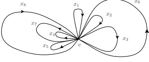
To define the sign function σ as in Sherman [2], we start with any planar drawing of an oriented
cotree, a graph with one vertex v andk loops corresponding to thek pairs of generators and their
inversex±11, . . . , x±k1. See Figure 2.1 as an example of cotree with eight loops. To each generatorxi can be associated the closed pathpithat traverses the corresponding loop, starting and terminating
atv, following the oriention of the loop; andx−i1 can be associated with the reverse pathp−i1. For a c-reduced word w = xe1
i1· · ·x
eℓ
iℓ, the sign σ(w) is defined as (−1)
r−1 where r is the number of
revolutions made by the tangent vector to the associated path pe1
i1· · ·p
eℓ
iℓ as the path is traversed.
Note that different drawings may give different sign functions.
For the definition of sign, it is convenient to assume the drawing of the graph is given so that
x1
x2
x3 x6
x4
x5 x7 x8
[image:19.595.174.432.458.566.2]v
Figure 2.1: Cotree with eight loops
the loops are represented by smooth closed curves with tangent vectors that vary continuously over
‘time’ as the loop is traversed, except perhaps at v, but where there is a limiting value at the
beginning and end of each loop. Ift1 (a unit vector in the plane) is the value of the tangent vector
as the path nears the end of one loop and t2 is the value of the tangent vector as the path begins
another loop, we must imagine a short time in which the tangent vector rotates fromt1 tot2 either
clockwise or counter-clockwise, whichever is the least motion, i.e. whichever motion goes through
(which case would arise, e.g., if the word were not c-reduced).
It is clear that the sign of a rotation of a c-reduced word is the same as the sign of the original
word. It is also clear thatσ(xi) =σ(x−i1) = +1 for any generatorxi. If the number of revolutions of the tangent vector made by traversing a pathqassociated with a c-reduced worduisr, then the
number of revolutions of the tangent vector made by traversingqd isdr, and so
σ(ud) = (−1)dr−1= (−1)d−1(−1)d(r−1)= (−1)d−1(σ(u))d.
This establishes (2.3) and (2.4).
Given a word w, let L(w) be the induced planar drawing of the set of loops corresponding to
the symbols in w. A loop in L(w) is extremal in L(w) when it either contains no other loops in
L(w), or contains all other loops inL(w). A symbola, which is one of the generatorsxi orx−i1, is
extremal in wwhen it occurs in wand its corresponding loop is extremal inL(w). For example, if
the drawing is as described in Figure 2.1 and w =x2
1x−83x6x8x2, then the extremal symbols inw arex1, x2, x8, x−81.
Lemma 2.3.1 Letabe a symbol in a c-reduced wordw, sayw=uakv, wherek
6
= 0and the symbols
on either side of a in the cyclic order are different froma. (That is, udoes not terminate with a,
andvdoes not terminate with awhenuis empty. Similarly, vdoes not begin withaandudoes not
begin withaif v is empty.) If ais an extremal symbol inw, then
σ(ua−kv) =−σ(uakv).
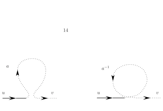
Proof. First consider the case whenk= 1. The diagrams in Figure 2.2, where we have suppressed the vertexv and made the paths continuous, are suggestive. It seems clear the trace of the tangent
vector around one of the paths has one more revolution than the other, so that the signs will differ.
But we should be careful, for example in the casec=b−1below.
u a−1
v
u v
[image:21.595.191.521.66.291.2]a
Figure 2.2: Illustrative graph for the change of revolution number
andcthe symbol that appears just aftera(at the beginning ofv, ifvis nonempty). It is important
that the loops corresponding tobandcare both outside or both inside the loop corresponding toa,
and this is ensured by our choice of aas extremal inw. We illustrate the case when they are both
outside. Label the anglesα,β,γ, andδas shown in Figure 2.3, all taken clockwise as positive. We
allowc=b−1, in which caseδ= 0.
The difference of the number of revolutions betweenuav andua−1v is
{β+γ−(π−α)}/2π− {−α−β−δ+ (π−γ−δ)}2π= 1
Figure 2.3 illustrates the case when all angles are smaller thanπ, but the calculation holds when
one of them is greater thanπ. For example, whenδis greater thanπ, it would be more intuitive to
write the difference as
{−(δ−π)}/2π− {−2π−(δ−π)}/2π
but sinceα+β+δ+γ= 2π, the result is the same. So the signs are different whenk= 1.
It is easy to see that σ(uakv) = (
−1)k−1σ(uav) andσ(ua−kv) = (
−1)k−1σ(ua−1v), for positive
integersk. Thus the theorem holds for anyk.
Proof of (2.5).Fixn1, . . . , nk with at leasttwoof the ni’s positive; letn=n1+· · ·+nk. LetS be the set ofc-reduced wordsw(not circular-words) in the free group generated byx1, . . . , xk with
b a
c
α
β
[image:22.595.239.420.143.306.2]γ δ
Figure 2.3: Illustrative graph for calculation of change of angles
φ:S →S, so thatσ(φ(w)) =−σ(w) for all w∈S.
Given a word c-reduced wordw∈S, leta=x±i1 be an extremal symbol inwwhose subscripti is the least so that the corresponding loop in extremal inL(w). Find the first occurrence of a term
ak inw and change it toa−k, and also change the exponent of any term aℓ at the end ofwin the case that wbegins witha, to getφ(w). For example, suppose the loops corresponding to x±11 and x±21 are the only extremal loops inL(w). Then
φ(x43x−22x−17x4) =x34x−22x71x4 and φ(x41x2−2x71x4x51) =x−14x−22x71x4x−15.
It is clear thatφ2 is the identity and by Lemma 2.3.1, we haveσ(φ(w)) =−σ(w).
Remark. Even though the sign of a word depends on the particular drawing, bothN(n1,· · ·, nk; +) andN(n1,· · · , nk;−) are independent of the drawing. Of courseW(n1,· · ·, nk; ) =W(n1,· · ·, nk; +)+
W(n1,· · · , nk;−) is independent of the drawing, and Lemma 2.3.1 shows that bothW(n1,· · ·, nk; +)
andW(n1,· · ·, nk;−) are independent of the drawing. Then by Lemma 2.2.1 and M¨obius inversion,
nN(n1, n2, . . . , nk; +) = X d|g, dodd
µ(d)W(n1 d,
n2 d, . . . ,
nk
nN(n1, n2, . . . , nk;−) = X d|g, dodd
µ(d)W(n1 d,
n2 d, . . . ,
nk
d ;−) − T, (2.13)
whereT = 0 whengis odd andT=W(n1
2, n2
2, . . . , nk
2 ;−) wheng is even. Hereµ(d) is the
number-theoretic M¨obius function. Therefore, N(n1,· · ·, nk; +) and N(n1,· · · , nk;−) are independent of
the drawing.
2.4
More on the sign function
The following lemma provides a combinatorial method for computing the sign of a word, with respect
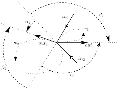
to any drawing of the cotree. Letw1 andw2 be c-reduced words. Fori= 1,2, let outi be a directed
line segment starting at v and in the direction of the tangent to the path coresponding towi as it
leavesv. Fori= 1,2, let ini be a directed line segment terminating atv and in the direction of the
tangent to the path corresponding to wi as it returns tov. There will be a circular order on the
four line segments atv. We say thatw1 andw2 interlacewhen in1 and in2 separate out1and out2
in this order. Figure 2.4 shows one type of interlacing.
Lemma 2.4.1 Ifw1andw2are c-reduced words so thatw1w2is also c-reduced, then, with the above notation,
σ(w1w2) = +σ(w1)σ(w2)
if w1 andw2 interlace, and
σ(w1w2) =−σ(w1)σ(w2)
otherwise.
Proof.First suppose thatw1andw2interlace and letα1,α2,β1, andβ2be the angles as indicated in Figure 2.4, as one of the possible situations. Others are similar and omitted. Let the number of
revolutions ofwi beri, and we separate it into two parts: 2πri= 2πri′+αi. Ifr12 is the number of
revolutions ofw1w2, start from out1, then 2πr12= 2πr′1+β1+2πr′2+β2Sinceα1+α2−β1−β2= 2π,
we getr12=r1+r2−1, which will yield the correct sign rule. Had we taken clockwise as positive
In the case when in1 is at the “bottom” and in2 is at the “top”, then the calculation would be
the same ifα1is still defined as the angle from in1to out1,β1the angle from in1to out2, and similar
forα2 andβ2. When w1 andw2 do not interlace, the proof is similar.
w1
out1 in1
in2 out2
w2
β2 α2
β1
[image:24.595.242.474.234.413.2]α1
Figure 2.4: Interlacing graph
Here is an example of the computation of σ(x1x2x3x4x5x6x7x8) when the cotree is as in Figure
2.1:
σ(x1x2x3x4x5x6x7x8) = (−)σ(x1x2x3x4x5x6x7)σ(x8)
= (−)(−)σ(x1x2x3x4x5x6)σ(x7)σ(x8)
=· · ·= (−)(−)(+)(−)(+)(+)(−) = +.
It is easy to see that every c-reduced word, involving at least two generators, can be written as the
product of two c-reduced words, so Lemma 2.4.1, used successively, allows the computation of the
sign of any word with respect to any drawing.
In case that the cotree is the “daisy”, as the example shown in Figure 2.5 below, in the case of
five loops, da Costa and Variane[5] have given an explicit rule to compute the sign of a c-reduced
D1 D2
D3
D4 D5
Figure 2.5: Daisy graph
Associated with each word w = Dei1
i1 D
ei2
i2 · · ·D
eil
il a sequence Sl = (i1, i2,· · · , il), where Dij’s
are symbols. Let s be the number of negative exponents eij’s. The sequence is such that a loop
ij appears at least once in S, for all j = 1,2,· · ·, l, andik 6=ik+1 andil 6=i1. DecomposeS into
T subsequences such that, each subsequence is an ordered set of numbers formed in the following
way: (a) ifp, qare two elements inside the subsequence andqcomes afterp, thenq > p; (b) a new
subsequence begins whenever this ordering is broken in the sequence by two adjacent elements not
satisfying (a).
For instance, a sequence with three loops andl= 14 is decomposed as follows, withT = 7:
S14= (12123213232312) = (12)(123)(2)(13)(23)(23)(12).
Theorem 2.4.2 (da Costa and Variane)Let N be the total number of symbols in w, then the sign of wisσ(w) = (−1)N+l+s+T+1.
Proof.Recall thatσ(Dei1
i1 ) = (−1)
ei1+1, whereD′
jsare the counterclockwise loops as in Figure 2.5,
we calculate the sign as we did in the previous example, and use induction on s and T. Whens= 0
andT = 1, all the pairs in the calculation interlace, so
σ(Dei1
i1 D
ei2
i2 · · ·D
eil
il ) = (+)
l−1σ(Dei1
i1 )· · ·σ(D
eil
il ) = (−1)
When s = 0 and there is one increment of T in the word, the sign will gain one extra factor
of (−1) from the non-interlacing case of Lemma 2.4.1, which yields the same sign rule as [5]. For
each increment ofs, which implies one of the loops is traversed in the opposite direction, then the
Chapter 3
3.1
Outline
In this chapter, we will switch to cycles in a general directed graphs. By combining with the result
in Chapter 2 and adapting the theorem in this chapter to the special case when there is only one
vertex, a method for deriving the analytic formula of the number of non-periodic cycles with positive
and negative signs is developed. If there are only two loops adjacent to the vertex, the formula first
appeared in Costa [4]. We use our method and derive the same expression as well in Appendix B.
3.2
The number of non-periodic cycles
Given a directed graph D which may contain multiple edges and loops, let E(D) be the set of all
edges ofD. Theorigin of an edgeeis the starting vertex and theendofeis the ending vertex. The
inverseInv(e) ofeis the set of edges whose origin and end is the end and origin ofe, respectively.
Ifeis a loop, thene∈Inv(e). Thesuccessor E(e) ofeis the set of edges whose origin is the end of
e. Ife is a loop, thenInv(e)⊂E(e). Theproper successor P(e) ofeis E(e)\Inv(e) wheneis not
a loop. Wheneis a loop, thenP(e) is the same as E(e) .
A pointed cycle p is a closed path inD with a specified starting edge, and a cycle [c] is the
equivalent class of cyclic permutations ofc. A (pointed) cycle is calledreduced if there is no
imme-diate reversal as it traverses through an edge that is not a loop. Since we consider the inverse of a
loop is the same as itself, it is ok that the reduced cycle traverses through a loop multiple times.
Only reduced cycles are considered, so we may omit the word when appropriate.
Let ρbe the cyclic permutation of the pointed cyclec=e1e2...ek, i.e. ρ(c) =eke1...ek−1, then
theperiod of a cycle [c] is the least positive integer t so that ρt(c) =c. A cycle [c] of lengthM is
said to be non-periodic when the period of [c] isM. A ℓ-cycle is a cycle of total lengthℓ, i.e., the
number of edges isℓ.
and0 otherwise. LetND(ℓ)be the number of non-periodic reducedℓ-cycles inD. Then
X
ℓ|M
ℓND(ℓ) =Tr(TM). (3.1)
Proof. To prove the lemma, we count the number of reduced pointed M-cycles in two different ways. First, given a divisor ℓ of M, a reduced pointedM-cycle wwith period ℓ may be obtained
as follows: Start with a representative c of a non-periodic reduced cycle [c] of lengthℓ and repeat
it M/ℓ times to get a reduced pointed cycle w =cM/ℓ. Note that the first ℓ cyclic permutations
w, ρ(W), ..., ρM/ℓ−1(w) are different pointed cycles. By the definition of ND(ℓ), we conclude that the number of pointedM-cycles isP
ℓ|MℓND(ℓ). Here is the other way of counting. Letaandbbe the edge ofD. The (a, b)thentry ofTM is
TM(a, b) = X ei1,ei2,...,eiM−1
t(a, ei1)t(ei1, ei2)...t(eiM−1, b),
which counts the number of M-paths from the origin of edge a to the end of edge b. Taking the
trace of TM will ensure that only closed paths are counted and every starting edge is taken into
account. Notice that a periodic cycle with periodℓ and total lengthM is also counted ℓ times in
Tr(TM) since , even though there areM entries, the number of different edges isℓ. For example, if
M = 6 andℓ= 3, then the 6-cycle, saye1e2e3e1e2e3, is counted once by each oft6(e1, e1),t6(e2, e2),
andt6(e3, e3).
Lemma 3.2.2 Let µ()be the Mobius function. Then
ND(M) = 1 M
X
ℓ|M µ(M
ℓ )T r(T
ℓ) (3.2)
Proof.By the Mobius inversion formula, we can invert (3.1) to get
M ND(M) =X ℓ|M
µ(M ℓ )T r(T
Theorem 3.2.3 DefineP as the set of non-periodic reduced cycles in a direct graphD and denote the length of its element [c]∈Pby |c|. Then
Y
[c]∈P
(1−u|c|) = det(I−uT) (3.4)
Proof. It will suffice to prove that the formal logarithms of both sides of (3.4) are equal. The logarithm of the left-hand side is
X
[c]∈P
∞
X
ℓ=1 u|c|ℓ
ℓ =
∞
X
M=1
X
ℓ|M 1 ℓND(
M ℓ )u
M,
where ND(M
ℓ ) has the same definition as above. The above equation comes from collecting terms
that have the same powerM.
The logarithm of the right-hand side is
log det(I−uT) = Trlog(I−uT) = Tr
∞
X
ℓ=1 (uT)ℓ
ℓ =
∞
X
M=1
Tr(TM)
M u
M.
Comparing the coefficient ofuM, we get the two sides of (3.1).
3.3
The number of non-periodic cycles with specified
occur-rences of edges
Given a directed graphD which may contain multiple edges and loops, letND(m1, m2, ..., m|E(D)|)
denote the number of non-periodic reduced cycles of length M = m1+m2+...+m|E(D)| which
containmi of edgeei for eachi= 1,2, ...,|E(D)|. In order to keep track of the edges, every edgeei
is assigned an indeterminatexi. DefineS as a square matrix whose entriess(ei, ej) is√xixj when
with two loops, then S=
x1 √x1x2
√x1x2 x2
.
Lemma 3.3.1 Let f(m1, m2, . . . , mk) be the coefficient of a monomial xm1
1 x m2
2 ...x mk
k in T r(SM),
whereM =m1+m2+· · ·+mk, andg is the g.c.d. ofm1, m2, ..., mk, then
X
ℓ|g M
ℓ ND( m1
ℓ , m2
ℓ , ..., mk
ℓ ) =f(m1, m2, . . . , mk). (3.5)
Proof.We count the number of reduced pointed cycles withmi occurrence of edgexi in two ways. First given a divisor ℓ ofg, a reduced pointed cycle w with period ℓ and mi occurrence of xi, for
all i’s, may be obtained as follows: Start with a representative c of a non-periodic reduced cycle
[c] of lengthM/ℓ and repeat it ℓ times to get a reduced pointed cycle w =cℓ. By the definition
of ND(m1
ℓ , m2
ℓ , ..., mk
ℓ ), we conclude that the number of pointed M-cycles with mi occurrence of
xi isP
ℓ|gMℓND( m1
ℓ , m2
ℓ , ..., mk
ℓ ). Here is the other way of counting. In T r(S
M), the coefficient of
a monomial xm1
1 x m2
2 ...x mk
k is the number of pointed reduced cycles with mi occurrence of xi, for
similar reasons as in Theorem 3.2.1.
Theorem 3.3.2 LetIc be the product of xi’s that corresponds to the edgesei traversed by the cycle
[c]. Then
Y
[c]∈P
(1−Ic) = det(I−S). (3.6)
Proof. This theorem is a generalization of Theorem 3.2.3 and the proof will follow a similar argu-ment. The logarithm of the left-hand side is
X
[c]∈P
∞ X ℓ=1 Iℓ p ℓ = X
m1,m2,...,mk
X
ℓ|g 1 ℓND(
m1 ℓ ,
m2 ℓ , ...,
mk ℓ )x
m1
1 xm22...xmkk
wheregis the greatest common divisor of allmi’s. Multiplying byM =m1+m2+...+mk, we get
the coefficient ofxm1
1 x m2
2 ...x mk
k equals the number of pointedM-cycles with mi
ℓ occurrence ofxifor
The logarithm of the right-hand side is
log det(I−S) = Trlog(I−S) =T r
∞
X
M=1 SM
M .
After multiplying by M, the coefficient of xm1
1 xm22...xmkk equals the number of pointed M-cycles.
This is because taking the trace will ensure the path is closed and different starting positions are
counted accordingly.
3.4
Non-periodic cycles with positive and negative signs in
the special case
The analytical expression of the numberN(m1, m2;±) of non-periodic cycles with signs in the special
case of two loops is known[4], but there is no general expression when there arekloops,k >2. Here
we derive it as follows.
From Lemma 3.3.1, we can reverse (3.5) and get
ND(m1, m2, ..., mk) =X d|g
µ(d)
M f(m1/d, m2/d, . . . , mk/d). (3.7)
In order to apply this result to the special case as in Chapter 2, the directed graph now is a single
vertex with loops embedded on a plane, and the inverse of the loop is always present and considered
as different from itself due to the two orientations; therefore, it has to be excluded from the proper
successor of itself. For example, the matrixSin the case of two loops, along with their inverse loops,
is
S=
x1 0 √x1x2 √x1x2
0 x1 √x1x2 √x1x2
√x1x2 √x1x2 x2 0
√x1x2 √x1x2 0 x2
. (3.8)
If we define WD(m1, m2, ..., mk) as the number of pointed reduced M-cycles in D with mi
occurrence of ei for i = 1,2, ..., k and M = m1 +m2 +...mk, then, by a similar argument as
Lemma 2.2.1, we get
WD(m1, m2, ..., mk) =X ℓ|g
M ℓ ND(
m1 ℓ ,
m2 ℓ , ...,
mk ℓ ),
whereND(m1
ℓ , m2
ℓ , ..., mk
ℓ ) is calculated in (3.7).
The subscript D is to signify that WD(m1, m2, ..., mk) applies to general directed graph. The
functionW(m1, m2, ..., mk;±), as defined in Chapter 2, applies to only the special case. Nonetheless,
when we treat the special case as a directed graph and define
W(m1, m2, ..., mk) =W(m1, m2, ..., mk; +) +W(m1, m2, ..., mk;−),
thenW(m1, m2, ..., mk) =WD(m1, m2, ..., mk).
Put together,
W(m1, m2, ..., mk) = WD(m1, m2, ..., mk)
= X
ℓ|g M
ℓ ND( m1
ℓ , m2
ℓ , ..., mk
ℓ ).
Substitute (3.7) into the above expression to get
X
ℓ|g M
ℓ (
X
d|g′
µ(d) M/ℓf(
m1 ℓd, ...,
mk ℓd)) =
X
p|g f(m1
p , ..., mk
p )
X
d′|p
µ(d′)
whereg′ is the greatest common divisor ofmi/ℓ. By using the property of the Mobi¨us Function:
X
d|n µ(d) =
1 if n = 1
we derive
W(m1, m2, ..., mk) =f(m1, ..., mk). (3.9)
The reason we introduce the functionWD(m1, m2, ..., mk) is to help us connect with the function
N(m1, m2, . . . , mk;±), which is defined in Chapter 2. Because
W(m1, m2, ..., mk; +) =W(m1, m2, ..., mk;−),
as proved in Chapter 2, we have
W(m1, m2, ..., mk; +) =W(m1, m2, ..., mk;−) =W(m1, m2, ..., mk)/2. (3.10)
If we replace W(m1, m2, ..., mk;±) in (2.12) and (2.13) by (3.10) and use W(m1, m2, ..., mk) =
f(m1, ..., mk), we have
N(m1, m2, . . . , mk; +) = X d|g, dodd
µ(d)
2M f(m1/d, m2/d, . . . , mk/d), (3.11)
and
N(m1, m2, . . . , mk;−) = X d|g, dodd
µ(d)
2M f(m1/d, m2/d, . . . , mk/d)
− T (3.12)
whereT = 0 wheng is odd andT =W(m1
2 , m2
2 , . . . , mk
2 ;−) wheng is even.
In principle, the function f(m1, ..., mk) can be calculated from its definition; therefore, we can
derive expressions forN(m1, m2, ..., mk; +) andN(m1, m2, ..., mk;−). We also show in Appendix A
Chapter 4
4.1
Introduction
We will apply the Feynman Identity to certain graphs to derive combinatorial identities involving
binomial numbers. A rigorous proof of each identity is provided separately.
The Feynman Identity can be presented as
X
G∈A
G(xi) =Y c∈P
(1 +Jc(xi)), (4.1)
where xi is the indeterminate corresponding to the edge ei,Ais the set of even simple subgraphs,
andG(xi) =Q
ix mi
i wheremi is the multiplicity ofeiin the subgraphG. SinceGis a simple graph,
mi here equals either one or zero, but in general it is some non-negative number. For simplicity,G
is used to denote both the subgraph inAand the corresponding monomial. On the right hand side,
c is a class of non-periodic paths and P is the set of equivalent classes up to the “starting point”
and orientation. For example, aC4 is a path that has four starting point and after accounting for
orientations, there are eight paths and they belong to the same class. Jc(xi) =σ(c)Q
ix mi
i where
mi is the multiplicity ofei inc andσ(c) is the sign of cas defined in Chapter 2.
For future reference, we will call the left hand side of (4.1) the graph side and the right hand
sidethe path side.
4.2
An alternative form of the Feynman Identity
The Feynman Identity can be rewritten by taking logarithm on both sides of (4.1) and comparing
the coefficient of the monomialQ
ix mi
i whereiruns over the non-zeromi’s. After taking logarithms,
the coefficient on the path side is again
1
M(W(m1, m2, ..., mk; +)−W(m1, m2, ..., mk;−)),
as in the special case in Chapter 2. This is because the relation between N(m1, ..., mk;±) and
valid as long as the graph is embedded in atwo-dimensional orientable manifold. The logarithm on
the graph side, after Taylor expansion, is
X
A\∅
G(xi)
−12 X
A\∅
G(xi)2
+1 3
X
A\∅
G(xi)3 −...=
∞
X
B=1
(−1)B+1 B
X
j
Gj(xi)B
(4.2)
where each of the summations on the left is over the setA\∅of non-empty even simple subgraphs.
So the identity can be rephrased as the following: Let [f(x1, x2, ..., xk)]xm1 1 x
m2 2 ...x
mk
k denote the
coefficient of the monomial termxm1
1 x m2
2 ...x mk
k in the polynomial f(x1, x2, ..., xk). Then
h X
A\∅
G(xi)
−12 X
A\∅
G(xi)2
+1 3
X
A\∅
G(xi)3 −...i
xm1 1 x
m2 2 ...xmkk
= 1
M W(m1, m2, ..., mk; +)−W(m1, m2, ..., mk;−)
. (4.3)
4.3
The first identity
The first identity we will derive is in the following theorem.
Theorem 4.3.1 Let y1, y2, ..., yL be positive intergers and X a positive number such thatX−1≥
PL
ℓ=1yℓ. Then
X
X
B=1
(−1)B+1 B
max{yi}
X
j=B
(−1)B+j
B j j y1 j y2 ... j yL
= 0, (4.4)
where the inner summation overj goes in a decreasing order. (The reason for the decreasing order
will become clear in the proof.)
Proof using the Feynman Identity. Define thedegree-star deg∗(vi) of a vertexvi as the number of edges incident with vi and counting multiple edges as 1. For example, if there are totally three
edges incident withvi but two of them are mulple edges, thendeg∗(vi) = 2. We will look into the
case whendeg∗(vi)≤2 for allvi’s.
Given a set of parameters {mi} which specifies the number of occurrence of each edge ei, let
equal to, say,m, then the path side of (4.3) has nonzero coefficient. In this case, both sides equal
(−1)(m+1)/m. This is explained in Appendix B.
When G{mi} is not connected, let the number of components be L. Since deg
∗(vi) ≤ 2 for
all vertices, each of the component Cℓ of G{mi} is actually a closed path repeated, say yℓ times,
ℓ= 1,2, ..., L, whereyℓ=mi ifei ∈Cl. Without lose of generality, lety1 ≥y2≥...≥yL ≥1. The
coefficient ofQ
ix mi
i in the term
P
A\∅G(xi)
B
is
y1
X
j=B
(−1)B+j
B
j
j
y1
j
y2
...
j
yL
. (4.5)
Notice that the summation over j goes in a decreasing order because we use inclusion-exclusion
principle, which is explained in the next paragraph.
The first term j=B comes from the following. First we chooseyℓ out ofB factors in the term
X
A\∅
G(xi)B
to compose the repeated component Cℓ. Because each individual factor contains subgraphs as
the direct composition of several Ci’s, we can choose them “without replacement”. But since the
summation overA\∅does not contain the empty graph, which corresponds to 1, each factor has to
contribute at least one component. We may use the inclusion-exclusion principle to get rid of those
terms that contribute less thanB factors.
The range of B for which the coefficient of Q
ix mi
i is nonzero goes fromy1, i.e., the maximum
of allyℓ’s, toP
ℓyℓ. The lower valuey1comes from the fact that the set A\∅contains only simple
graphs without repeated edges, so we need at least y1 factors to compose C1 repeated y1 times.
The upper value comes from the fact that, if each factor contributes exactly one component, which
is the most “spread-out” situation, then the total number of factors equals the total number of
components, counting multiplicities, which isP
The above expression in (4.5) is the coefficient of Q
ix mi
i from the term
P
A\∅G(xi)
B
. If we
sum over allB’s, then the left hand side of (4.3) becomes
X
X
B=1
(−1)B+1 B
y1
X
j=B
(−1)B+j
B j j y1 j y2 ... j yL , (4.6)
whereX is some finite number such that all nonzero terms are taken into account. WhenBis larger
thanP
ℓyℓ, because each factor of the term
P
A\∅G(xi)
B
has nonzero contribution and totally
we need only P
ℓyℓ, the coefficient from the term
P
A\∅G(xi)
B
has to be zero. Therefore the
inner summation overj in (4.6) becomes zero when B is larger thanP
ℓyℓ. This is the expression
we get from the graph side.
We can see easily that the path side of (4.3) is zero. Since G{mi} is not connected, there is no
way to traverse it in one stroke. So bothW(mi; +) andW(mi;−) are zero.
Alternative proof. Since for allj < y1, the expression (4.5) is zero, we rewrite the summation indexj as from 1 to B. After interchanging the order of summation, we have
X X B=1 1 B B X j=1
(−1)j+1
B j j y1 j y2 ... j yL = X X j=1 X X B=j 1 B B j
(−1)j+1
j y1 j y2 ... j yL . (4.7)
By using the identity (1.52) in [8], the inner summation on the right hand side of (4.7) can be written
as X X B=j 1 B B j = X X B=j j
B−1 j−1
=j X j =X
X−1 j−1
.
Subsituting back into (4.7), we get
X
X
j=1
(−1)j+1X
X −1 j−1
j y1 j y2 ... j yL =X X−1
X
k=0 (−1)k
X−1 k
k+ 1 y1
k+ 1 y2
...
k+ 1 yL
Use the identity (x.16) in [8]
n
X
k=0 (−1)k
n
k
a1+b1k
m1
a2+b2k
m2
...
ar+brk
mr
= 0, (4.9)
with the condition 0≤m1+m2+...+mr ≤n. Substitute with n=X −1,r=L,mi=yi, and
ai=bi= 1 for alliin (4.9) to see that this is exactly the expression in (4.8). The condition onX is
also satisfied sinceX−1≥P
yi, so the expression in (4.4) is zero.
This complete the prove of the first theorem. We make some preliminary remarks before we state
the second theorem.
4.4
A combinatorial lemma
Suppose there are A different objects, A ≥ 2, and R of them are special. We want to partition
them into B different baskets with the following rule: (1) None of the basket are empty and (2)
theR special objects arein different baskets. Only whenB ≤A can the first rule be satisfied and
only whenR≤B can the second one be satisfied; so the number of partition is nonzero only when
R≤B ≤A.
A real life example may be, during Easter, we want to put R eggs into different baskets. None of
the eggs are the same but we want to have at most one egg in each basket. The rest of the objects
are candies and they can go to any basket. All the baskets must be nonempty.
We can partition the Aobjects in the following way. To partition the R special objects, or the
eggs in the previous example, chooseRbaskets out ofB, so there are BR
R! ways of partition. Take
J objects out of the rest of theA−R objects, which are thecandies in the previous example, and
fill up the rest of the B−R baskets. Since none of them is allowed to be empty, J ≥B−R. The
rest of theA−R−J objects then can go into any of the firstR baskets. LetF(N, k) denote the
of the partitions of the candies is
A−R
X
J=B−R
A −R J
F(J, B−R)RA−R−J.
Combined together, the total number of distribution, denoted byD(A, R;B), is
D(A, R, B) =
B R
R! A−R
X
J=B−R
A−R J
F(J, B−R)RA−R−J. (4.10)
Notice that each term in the summation is mutually exclusive due to the total number of candies
in the no-egg baskets. If we denote the Stirling numbers of the second kind by S2(N, k), which
is the number of distributions of N different objects into k identical baskets, thenF(J, B−R) =
(B−R)!S2(J, B−R).
Here is an interesting identify aboutD(A, R;B).
Lemma 4.4.1 Based on the definition ofD(A, R;B) and with the condistion thatA > R,
A
X
B=R
(−1)B+1
B D(A, R;B) = 0. (4.11)
Proof.Let the above summation beG(A, R) and substitute the expression forD(A, R;B) in (4.10) into (4.11) to obtain
G(A, R) = A
X
B=R
(−1)B+1 B B R R! A−R
X
J=B−R
A−R J
F(J, B−R)RA−R−J.
ReplaceF(J, B−R) by (B−R)!S2(J, B−R) and rearrange the terms to get
G(A, R) =RA−R A
X
B=R A−R
X
J=B−R
(−1)B+1 B B!
A −R
J
Interchange the two summations along with the proper summation ranges to get
G(A, R) =RA−R A−R
X
J=0 R+J
X
B=R
(−1)B+1(B−1)!S2(J, B−R)
A −R
J
R−J.
Letb=B−R and put those terms related tob together:
G(A, R) =RA−R(−1)R+1 A−R
X
J=0
A−R J
R−J J
X
b=0
(−1)b(b+R−1)!S2(J, b).
The second summation can be simplified using the generating function of S2, which we will prove
later:
J
X
b=0
(−1)b(b+R−1)!S2(J, b) = (−R)J(R−1)!. (4.12)
Therefore,
G(A, R) =RA−R(−1)R+1 A−R
X
J=0
A−R J
R−J(−R)J(R−1)!.
Notice thatR−J(−R)J = (−1)J, so the part of summation overJ becomes
A−R
X J=0 A −R J
(−1)J = (1
−1)A−R= 0.
This completes the proof of (4.11). To finish the story we come back to (4.12) and use the
generating function of the Stirling numbers of the second kind:
xJ= J
X
b=0
S2(J, b)x(x−1)...(x−b+ 1). (4.13)
Letx=−Rin (4.13) and notice there areb terms followingS2(J, b) on the right-hand side:
(−R)J = J
X
b=0
Complete the factorial by multiplying both sides by (R−1)!. Then (4.14) becomes (4.12):
(−R)J(R−1)! = J
X
b=0
(−1)b(R+b−1)!S2(J, b).
4.5
The second identity
Recall that G{mi} is the graph with edge ei of multiplicity mi. A repeated edge is one that has
multiplicity greater than one. We can decomposeG{mi} into a set of subpathsS ={pj} such that
(1) the degrees of the vertices ofpj all equal two for allj and (2) thedisjoint union of the edge set
E(pj) isE(G{mi}); here disjoint means that the repeated edges in different edge set is not eliminated
as we combine them together. DefineA as the number of paths inS, i.e.,A=|S|, and notice that
A≥2 when there exists at least one vertexvj withdeg∗(vj)>2.
Use adecomposition matrix SA×|E(G{mi})|to denote the decomposition whereSi,j= 1 when the
sub-path pi resulting from the decomposition S contains edge ej andSi,j = 0 otherwise. Given a graphG{mi}, there may be different ways of decomposition that satisfy the above rule, and we will
use a subcript, i.e.,Si to denote the set andSito denote the matrix when necessary.
After the decomposition, there areAsubpaths, and it is desired to partition them into B parts,
which we will call theegg-candy partition procedure (the name is inspired from the Easter example in
the previous section): Partition the elements of the setSintoB parts and put them intoBdifferent
baskets such that no two subgraphs in the same basket have common edges. This way, the direct
composition of the subpaths in the same basket corresponds to a unique even subgraph in the term
P
jGj(xi). Therefore, each choice of the above procedure contributes 1 to the coefficient of
Q
ix mi
i .
In view of the Easter example, those subpaths that have common edges are treated as eggs with
common features, and they are not supposed to go to the same basket; eggs that have no features in
common then can go to the same basket. Those subpaths without any repeated edges are candies
For example, ifS={p1, p1, p2, p2}wherep1 andp2 do not have any common edge, so p1 andp2
are different kinds of eggs, but the twop1’s are considered the same kind of eggs. IfB = 2, then the
only elligible partition is to putp1 andp2 into the same basket, and repeat it again for the second
basket. Therefore the term (P
jGj(xi))B contribute 1 to the coefficient of
Q
ix mi
i when B = 2.
This is because one can always find the unique subgraph, sayGj, which has exactly the same edge
set as the disjoint union ofE(p1) andE(p2) and the same subpaths cannot be put together in the
same basket since the subgraphs are simple ones. If B = 3, There are 3! different ways to assign
{{p1, p2},{p1},{p2}}into three different basket, so the total contribution is 3!. IfB= 4, then there
are 4!/2!2! different partitions. Ifp1 andp2have any edge in common, then the total is 4!/2!2! when
B= 4 and zero otherwise.
LetD(S;B) be the coefficient ofQ
ix mi
i in the term
P
jGj(xi)
B
contributed from the
decom-position S. For example, take S ={p1, p1, p2, p2} in the above paragraph where p1 and p2 don’t
have any common edge, thenD(S; 2) = 1, D(S; 3) = 3, andD(S; 4) = 6.
Theorem 4.5.1 Suppose the decompositionS is such that the matrix Shas only one column with more than one nonzero entry, i.e., there is only one edge ei with mi =R >1, and the other mi’s
equal 1. Then
A
X
B=R
(−1)B+1
B D(S;B) = 0, (4.15)
whereA is the number of rows ofS.
Proof using the Feynman Identity. Based on the discussion ofD(S;B), the coefficient ofQ
ix mi
i
on the graph side of (4.3) is
∞
X
B=1
(−1)B+1
B D(S;B).
So the alternative form of the Feynman Identity becomes
∞
X
B=1
(−1)B+1
B D(S;B) = 1
M W(m1, m2, ..., mk; +)−W(m1, m2, ..., mk;−)
. (4.16)
(4.15) on the left hand side.
We know that if there is any repeated edge, then the path side of the Feynman Identity (4.3)
is zero. To be specific, because the paths are not allowed to go backward immediately, we can
shrink the repeated edgeeR by connecting the vertices ofeRas a single vertex, and the situation is
equivalent to the special case when there is a single vertex with several loops; therefore, we have a
one-to-one mapping between the positive- and negative-sign paths.
Alternative proof. In the case when the decompositionS produces|A| subpaths andRof them have a common repeated edge, and there is no other repeated edge,D(S;B) is the same asD(A, R;B)
in the previous section. Again, the nonzero term starts fromB =Rand ends atB=A, as explained
in the previous section. So the graph side of the Feynman Identity is same as the left hand side of
(4.11) in Lemma 4.4.1. By Lemma 4.4.1, we know that this expression is zero.
4.6
Two more combinatorial lemmas
Lemma 4.6.1 Let mbe a positive integer and xis a positive number. Then
m
X
k=0
(−1)k m+x+k
m+x+k k
m+x m−k
= 0 (4.17)
Proof.Consider the first term whenk= 0. The left hand side of (4.17) can be written as
Xm
k=1
(−1)k m+x+k
m+x+k
k
m+x
m−k
+ 1
m+x
m+x
0
m+x
m
.
So we will prove that
m
X
k=1
(−1)k m+x+k
m+x+k k
m+x m−k
= −1 m+x
m+x m
Use n t = n t n −1 t−1
, (4.19)
to get
1 m+x+k
m+x+k k
= 1 k
m+x+k−1 k−1
.
So the summation in (4.18) becomes
m
X
k=1 (−1)k
k
m+x+k −1 k−1
m+x
m−k
. (4.20)
We need to deal with (−1)k. Using the definition
−z
k
= 1
k(−z)(−z−1)...(−z−k+ 1),
we get the following identity:
−z
k
= (−1)k
z+k−1 k
. (4.21)
So
(−1)(k−1)
m+x+k+ 1
k−1
= (−1)(k−1)
(m+x+ 1) + (k
−1) + 1 k−1
=
−(m+x+ 1) k−1
.
Substitute this expression back into the summation in (4.20), the expression (4.18) becomes
m
X
k=1 (−1)k
k
m+x+k−1) k−1
m+x m−k
= m X k=1 −1 k
−(m+x−1) k−1
m+x m−k
.
Using (4.19) again withn=−(m+x) andt=k, we get
m
X
k=1
−1
−(m+x)
−(m+x) k
m+x
m−k
= 1
(m+x) m
X
k=1
−(m+x) k
m+x
m−k
If we add and subtract the termk= 0, we get
1 (m+x)
Xm
k=0
−(m+x)) k
m+x
m−k
−
−(m+x) 0
m+x
m . Using m X k=0 a k b m−k
=
a+b m
, (4.22)
which is true for generalaand b, we see that the first summation becomes m0
, which equals zero.
So put together, the left hand side of (4.18) becomes
1 (m+x)
0−
−(m+x) 0
m+x
m
= −1 m+x
m+x
m
,
which is the right hand side of (4.18)
Lemma 4.6.2 Let mbe a positive integer and xa positive number. Then
m
X
k=0 (−1)k
m+x+k−1 k
m+x m−k
= 0. (4.23)
Proof.We will use (4.21) again to get
(−1)k
m+x+k −1 k
=
−(m+x) k
.
So the summation becomes
m
X
k=0 (−1)k
m+x+k−1 k
m+x m−k
= m X k=0
−(m+x) k
m+x m−k
,
which is zero by (4.22).
4.7
The third identity
Suppose that after the decomposition, every subpath contains exactly one repeated edge. For
ex-ample, ifp1, p2, and p3 have the common edgee1, andp4,p5 have the common edgee2, then the
upper left part of the decomposition matrixSlooks like the following:
1 0 · · ·
1 0 · · ·
1 0 · · ·
0 1 · · ·
0 1 · · ·
0 0 · · ·
.. . ... ...
Let the multiplicity of edge ei be Ri, i = 1,2, ..., n, and let the coefficient in the Bth term
(P
jGj(xi))B beD(R1, R2, ..., Rn;B). We useD(R1, R2, ..., Rn;B) instead ofD(S;B) since we will
need the recursion relation onn. Without loss of generality, letR1≥R2≥...≥Rn≥2.
Theorem 4.7.1 Let D(R1, R2, ..., Rn;B)be defined as in the last paragraph. Then
R1+R2+...+Rn
X
B=R1
(−1)B+1
B D(R1, R2, ..., Rn;B) = 0. (4.24)
Proof using the Feynman Identity. Since the expression for the coefficient of Q
ix mi
i is
D(R1, R2, ..., Rn;B), the left hand side of (4.24) is the same as the graph side of (4.3). Again,
the nonzero terms start fromB=R1 toB=A. Also we know that the whenever there is repeated
edge, the path side of the Feynman Identity yields zero. Therefore, the summation result is zero.
Alternative proof. We will prove the identity using induction, and the base case is whenn= 2. For simplicity of notation, we will use (4.25), an expression forD(R1, R2;B), to prove (4.24) when
Here is the expression forD(R1, R2;B):
D(R1, R2;B) =
B
R1
R1!
R2
B−R1
(B−R1)!
R1
R2−(B−R1)
(R2−(B−R1))!. (4.25)
This is because to put R1+R2 objects into B non-empty different baskets, where only for B =
R1, R1+ 1, ..., R1+R2 is the expression nonzero, such that none of the first kind ofR1 objects are
in the same basket, and neither are the second kind of R2 objects, we chooseR1 out ofB baskets
and fill them with the first R1 objects. Since the baskets are different, we need the factor of R1!.
Then we chooseB−R1 out ofR2 second kind of objects and put into the rest of the baskets. For
the restR2−(B−R1) second kind of objects, they need to go into the baskets filled with the first
kind of objects.
We can prove (4.24) in the case whenn= 2 by substituting (4.25) into the summation in (4.24).
Letk=B−R1. Then (4.24) becomes
R1+R2
X
B=R1
(−1)B+1
B D(R1, R2;B)
= R1+R2
X
B=R1
(−1)B+1 B B R1 R1! R2 B−R1
(B−R1)!
R1 R2−(B−R1)
(R2−(B−R1))!
= R2
X
k=0
(−1)k+R1+1
R1+k
R1+k
R1 R1! R2 k k! R1
R2−k
(R2−k)!. (4.26)
In view of
R2 k
k!(R2−k)! =R2!,
the expression (4.26) becomes
(−1)R1+1R1!R2!
R2
X
k=0 (−1)k R1+k
R1+k
k
R1
R2−k
. (4.27)
Using (4.17) again from Lemma 4.6.1 and substituting withm=R2 andx=R1−R2, we see that
the expression (4.27) is zero.
relation
D(R1, ..., Rn;B) =Rn! B
X
i=B−Rn
B
i
i
Rn−(B−i)
D(R1, ..., Rn−1;B). (4.28)
We can easily understand (4.35) from the recursion relation betweenD(R1, R2, R3;B) andD(R1, R2;B):
D(R1, R2, R3;B) =R3! B
X
i=B−R3
B i
i R3−(B−i)
D(R1, R2;i). (4.29)
Choose i out of B baskets to put the first and second kind of objects, which is accounted by
D(R1, R2;i), and the remaining B−i baskets have to be filled up with the third kind of objects.
Now there areR3−(B−i) third kind of objects left. ChooseR3−(B−i) out ofibaskets which
already contain the first and/or the second kinds of objects. Since the baskets and the objects are
different, there is a factor ofR3!.
Now we will prove
R1+R2+R3
X
B=R1
(−1)B+1
B D(R1, R2, R3;B) = 0 (4.30)
and the proof for generalnis similar.
Substitute (4.29) into the left hand side of (4.30) and interchange the two summations:
R1+R2+R3
X
B=R1
(−1)B+1
B D(R1, R2, R3;B)
=
R1+R2+R3
X
B=R1
(−1)B+1 B R3!
B
X
i=B−R3
B i
i R3−(B−i)
D(R1, R2;i)
= R1−1
X
i=R1−R3
i+R3
X
B=R1
+ R1+R2
X i=R1 i+R3 X B=i +
R1+R2+R3
X
i=R1+R2+1
R1+R2+R3
X
B=i
(−1)B+1 B B i i R3