Treebank transfer

Treebank Transfer

Martin Jansche

Center for Computational Learning Systems Columbia University

New York, NY 10027, USA [email protected]

Abstract

We introduce a method for transferring annotation from a syntactically annotated corpus in a source language to a target lan-guage. Our approach assumes only that an (unannotated) text corpus exists for the target language, and does not require that the parameters of the mapping between the two languages are known. We outline a general probabilistic approach based on Data Augmentation, discuss the algorith-mic challenges, and present a novel algo-rithm for sampling from a posterior distri-bution over trees.

1 Introduction

Annotated corpora are valuable resources for Natu-ral Language Processing (NLP) which often require significant effort to create. Syntactically annotated corpora – treebanks, for short – currently exist for a small number of languages; but for the vast majority of the world’s languages, treebanks are unavailable and unlikely to be created any time soon.

The situation is especially difficult for dialectal variants of many languages. A prominent exam-ple is Arabic: syntactically annotated corpora ex-ist for the common written variety (Modern Stan-dard Arabic or MSA), but the spoken regional di-alects have a lower status in written communication and lack annotated resources. This lack of dialect treebanks hampers the development of syntax-based NLP tools, such as parsers, for Arabic dialects.

On the bright side, there exist very large anno-tated (Maamouri et al., 2003, 2004a,b) corpora for

Modern Standard Arabic. Furthermore, unannotated text corpora for the various Arabic dialects can also be assembled from various sources on the Internet. Finally, the syntactic differences between the Ara-bic dialects and Modern Standard AraAra-bic are rela-tively minor (compared with the lexical, phonologi-cal, and morphological differences). The overall re-search question is then how to combine and exploit these resources and properties to facilitate, and per-haps even automate, the creation of syntactically an-notated corpora for the Arabic dialects.

We describe a general approach to this problem, which we call treebank transfer: the goal is to project an existing treebank, which exists in a source language, to a target language which lacks annotated resources. The approach we describe is not tied in any way to Arabic, though for the sake of concrete-ness one may equate the source language with Mod-ern Standard Arabic and the target language with a dialect such as Egyptian Colloquial Arabic.

We link the two kinds of resources that are avail-able – a treebank for the source language and an unannotated text corpus for the target language – in a generative probability model. Specifically, we construct a joint distribution over source-language trees, target-language trees, as well as parameters, and draw inferences by iterative simulation. This al-lows us to impute target-language trees, which can then be used to train target-language parsers and other NLP components.

Our approach does not require aligned data, unlike related proposals for transferring annota-tions from one language to another. For exam-ple,Yarowksy and Ngai(2001) consider the transfer of word-level annotation (part-of-speech labels and bracketed NPs). Their approach is based on aligned

corpora and only transfers annotation, as opposed to generating the raw data plus annotation as in our ap-proach.

We describe the underlying probability model of our approach in Section 2 and discuss issues per-taining to simulation and inference in Section 3. Sampling from the posterior distribution of target-language trees is one of the key problems in iterative simulation for this model. We present a novel sam-pling algorithm inSection 4. Finally inSection 5we summarize our approach in its full generality.

2 The Probability Model

Our approach assumes that two kinds of resources are available: a source-language treebank, and a target-language text corpus. This is a realistic assumption, which is applicable to many source-language/target-language pairs. Furthermore, some knowledge of the mapping between source-language syntax and target-language syntax needs to be incor-porated into the model. Parallel corpora are not re-quired, but may help when constructing this map-ping.

We view the source-language treebank as a se-quence of trees S1, . . . ,Sn, and assume that these trees are generated by a common process from a corresponding sequence of latent target-language trees T1, . . . ,Tn. The parameter vector of the pro-cess which maps target-language trees to source-language trees will be denoted byΞ. The mapping itself is expressed as a conditional probability distri-bution p(Si|Ti,Ξ)over source-language trees. The parameter vectorΞis assumed to be generated ac-cording to a prior distribution p(Ξ|ξ) with hyper-parameterξ, assumed to be fixed and known.

We further assume that each target-language tree Ti is generated from a common language model Λ for the target language, p(Ti|Λ).For expository rea-sons we assume thatΛis a bigram language model over the terminal yield (also known as the fringe) of Ti. Generalizations to higher-order n-gram models are completely straightforward; more general mod-els that can be expressed as stochastic finite au-tomata are also possible, as discussed inSection 5. Let t1, . . . ,tkbe the terminal yield of tree T . Then

p(T |Λ) =Λ(t1|#) k

∏

Λ(tj|tj−1)

!

Λ($|tk),

where # marks the beginning of the string and $ marks the end of the string.

There are two options for incorporating the lan-guage model Λ into the overall probability model. In the first case – which we call the full model –

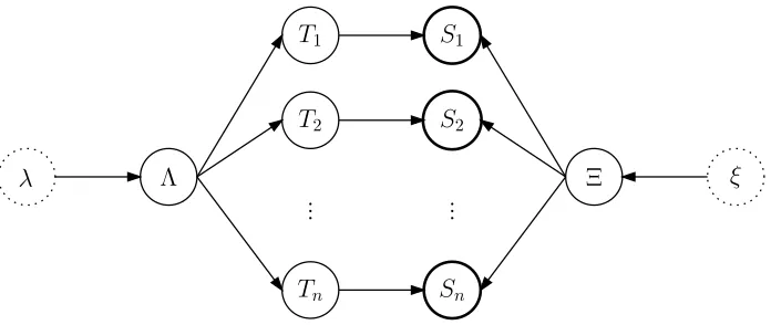
Λ is generated by an informative prior distribution p(Λ|λ)with hyper-parameterλ. In the second case – the reduced model – the language modelΛis fixed. The structure of the full model is specified graph-ically in Figure 1. In a directed acyclic graphical model such as this one, we equate vertices with ran-dom variables. Directed edges are said to go from a parent to a child node. Each vertex depends directly on all of its parents. Any particular vertex is condi-tionally independent from all other vertices given its parents, children, and the parents of its children.

The portion of the full model we are interested in is the following factored distribution, as specified by

Figure 1:

p(S1, . . . ,Sn,T1, . . . ,Tn,Λ,Ξ|λ,ξ)

=p(Λ|λ)p(Ξ|ξ) n

∏

p(Ti|Λ)p(Si|Ti,Ξ) (1)

In the reduced model, we drop the leftmost term/ vertex, corresponding to the prior forΛwith hyper-parameterλ, and condition onΛinstead:

p(S1, . . . ,Sn,T1, . . . ,Tn,Ξ|Λ,ξ)

=p(Ξ|ξ) n

∏

p(Ti|Λ)p(Si|Ti,Ξ) (2)

The difference between the full model(1)and the reduced model(2)is that the reduced model assumes that the language model Λis fixed and will not be informed by the latent target-language trees Ti. This is an entirely reasonable assumption in a situation where the target-language text corpus is much larger than the source-language treebank. This will typ-ically be the case, since it is usually very easy to collect large corpora of unannotated text which ex-ceed the largest existing annotated corpora by sev-eral orders of magnitude. When a sufficiently large target-language text corpus is available,Λis simply a smoothed bigram model which is estimated once from the target-language corpus.

λ Ξ ξ S1

T1

Λ

T2 S2

Tn Sn

... ...

Figure 1: The graphical structure of the full probability model. Bold circles indicate observed variables, dotted circles indicate parameters.

model is simply a discrete collection of multinomial distributions. A simple prior for Λ takes the form of a product of Dirichlet distributions, so that the hyper-parameterλ is a vector of bigram counts. In the full model(1), we assumeλ is fixed and set it to the observed bigram counts (plus a constant) in the target-language text corpus. This gives us an infor-mative prior for Λ. If the bigram counts are suffi-ciently large,Λwill be fully determined by this in-formative prior distribution, and the reduced model

(2)can be used instead.

By contrast, usually very little is known a pri-ori about the syntactic transfer modelΞ. InsteadΞ needs to be estimated from data. We assume thatΞ too is a discrete collection of multinomial distribu-tions, governed by Dirichlet priors. However, unlike in the case of Λ, the priors for Ξare nontive. This is not a problem, since a lot of informa-tion about the target language is provided by the lan-guage modelΛ.

As one can see in Figure 1 and equation (1), the overall probability model constrains the latent target-language trees Tiin two ways: From the left, the language modelΛserves as a prior distribution over target-language trees. On the one hand, Λ is an informative prior, based on large bigram counts obtained from the target-language text corpus; on the other hand, it only informs us about the fringe of the target-language trees and has very little di-rectly to say about their syntactic structure. From the right, the observed source-language trees constrain the latent target-language trees in a complementary

fashion. Each target-language tree Tigives rise to a corresponding source-language tree Si according to the syntactic transfer mappingΞ. This mapping is initially known only qualitatively, and comes with a noninformative prior distribution.

Our goal is now to simultaneously estimate the transfer parameterΞand impute the latent trees Ti. This is simplified by the following observation: if T1, . . . ,Tn are known, then finding Ξ is easy; vice versa, if Ξ is known, then finding Ti is easy. Si-multaneous inference forΞand T1, . . . ,Tnis possible via Data Augmentation (Tanner and Wong, 1987), or, more generally, Gibbs sampling (Geman and Ge-man,1984).

3 Simulation of the Joint Posterior

Distribution

We now discuss the simulation of the joint poste-rior distribution over the latent trees T1, . . . ,Tn, the transfer model parameterΞ, and the language model parameterΛ. This joint posterior is derived from the overall full probability model(1). Using the reduced model(2)instead of the full model amounts to sim-ply omittingΛfrom the joint posterior. We will deal primarily with the more general full model in this section, since the simplification which results in the reduced model will be straightforward.

language model Λ. It is possible to simulate this joint posterior distribution using simple sampling-based approaches (Gelfand and Smith,1990), which are instances of the general Markov-chain Monte Carlo method (see, for example,Liu,2001).

Posterior simulation proceeds iteratively, as fol-lows. In each iteration we draw the three kinds of random variables – latent trees, language model pa-rameters, and transfer model parameters – from their conditional distributions while holding the values of all other variables fixed. Specifically:

• Initialize Λ and Ξ by drawing each from its prior distribution.

• Iterate the following three steps:

1. Draw each Ti from its posterior distribu-tion given Si,Λ, andΞ.

2. Draw Λ from its posterior distribution given T1, . . . ,Tnandλ.

3. Draw Ξ from its posterior distribution given S1, . . . ,Sn, T1, . . . ,Tn, andξ.

This simulation converges in the sense that the draws of T1, . . . ,Tn, Λ, and Ξ converge in distribution to the joint posterior distribution over those variables. Further details can be found, for example, in Liu, 2001, as well as the references cited above.

We assume that the bigram modelΛis a family of multinomial distributions, and we write Λ(tj |tj−1) for the probability of the word tj following tj−1. Using creative notation, Λ(· |tj−1) can be seen as a multinomial distribution. Its conjugate prior is a Dirichlet distribution whose parameter vectorλw are the counts of words types occurring immediately after the word type w of tj−1. Under the conven-tional assumptions of exchangeability and indepen-dence, the prior distribution forΛis just a product of Dirichlet priors. Since we employ a conjugate prior, the posterior distribution ofΛ

p(Λ|S1, . . . ,Sn,T1, . . . ,Tn,Ξ,λ,ξ)

=p(Λ|T1, . . . ,Tn,λ) (3) has the same form as the prior – it is likewise a prod-uct of Dirichlet distributions. In fact, for each word type w the posterior Dirichlet density has parameter λw+cw, whereλwis the parameter of the prior distri-bution and cwis a vector of counts for all word forms

appearing immediately after w along the fringe of the imputed trees.

We make similar assumptions about the syntactic transfer modelΞand its posterior distribution, which is

p(Ξ|S1, . . . ,Sn,T1, . . . ,Tn,Λ,λ,ξ)

=p(Ξ|S1, . . . ,Sn,T1, . . . ,Tn,ξ). (4)

In particular, we assume that syntactic transfer in-volves only multinomial distributions, so that the prior and posterior for Ξ are products of Dirichlet distributions. This means that sampling Λ and Ξ from their posterior distributions is straightforward. The difficult part is the first step in each scan of the Gibbs sampler, which involves sampling each target-language latent tree from the corresponding posterior distribution. For a particular tree Tj, the posterior takes the following form:

p(Tj|S1, . . . ,Sn,T1, . . . ,Tj−1,Tj+1, . . . ,Tn,Λ,Ξ,λ,ξ)

=p(Tj|Sj,Λ,Ξ) =

p(Tj,Sj|Λ,Ξ)

∑Tj p(Tj,Sj|Λ,Ξ) ∝p(Tj|Λ)p(Sj|Tj,Ξ) (5)

The next section discusses sampling from this poste-rior distribution in the context of a concrete example and presents an algorithmic solution.

4 Sampling from the Latent Tree Posterior

C

S 1

v 2

O 3

a1 1

n1 2

a2 1

n2 2

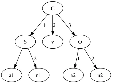
Figure 2: Syntax tree illustrating SVO constituent order within a sentence, and prenominal adjectives within noun phrases.

should be finite and representable as a packed for-est. More specifically, we assume that there is a compact (polynomial space) representation of po-tentially exponentially many trees. Moreover, each tree in the packed forest has an associated weight, corresponding to its likelihood under the syntactic transfer model.

If we rescale the weights of the packed forest so that it becomes a normalized probabilistic context-free grammar (PCFG), we can sample from this new distribution (corresponding to the normalized likeli-hood) efficiently. For example, it is then possible to use the PCFG as a proposal distribution for rejection sampling.

However, we can go even further and sample from the latent tree posterior directly. The key idea is to intersect the packed forest with the n-gram language model and then to normalize the re-sulting augmented forest. The intersection opera-tion is a special case of the intersecopera-tion construcopera-tion for context-free grammars and finite automata (Bar-Hillel et al.,1961, pp. 171–172). We illustrate it here for a bigram language model.

Consider the tree in Figure 2 and assume it is a source-language tree, whose root is a clause (C) which consists of a subject (S), verb (v) and object (O). The subject and object are noun phrases consist-ing of an adjective (a) and a noun (n). For simplicity, we treat the part-of-speech labels (a, n, v) as termi-nal symbols and add numbers to distinguish multiple occurrences. The syntactic transfer model is stated as a conditional probability distribution over

source-language trees conditional on target source-language trees. Syntactic transfer amounts to independently chang-ing the order of the subject, verb, and object, and changing the order of adjectives and nouns, for ex-ample as follows:

p(SvO|SvO) =Ξ1

p(SOv|SvO) = (1−Ξ₁)Ξ2 p(vSO|SvO) = (1−Ξ₁) (1−Ξ₂)

p(SvO|SOv) =Ξ3

p(SOv|SOv) = (1−Ξ3)Ξ4 p(vSO|SOv) = (1−Ξ3) (1−Ξ4) p(SvO|vSO) =Ξ5

p(SOv|vSO) = (1−Ξ₅)Ξ6 p(vSO|vSO) = (1−Ξ₅) (1−Ξ₆)

p(an|an) =Ξ7 p(na|an) =1−Ξ7 p(an|na) =Ξ8 p(na|na) =1−Ξ₈

Under this transfer model, the likelihood of a target-language tree[Av[Sa1n1][On2a2]]corresponding to the source-language tree shown inFigure 2isΞ5×

C

C_1

C_2 C_3

S

1 VO

2

S_1 S_2

a1 1

n1 2 2 1

v 1

O 2

O_1 O_2

a2 1

n2 2 2 1 1 OV

2

2 1

1 SO

2

1 2

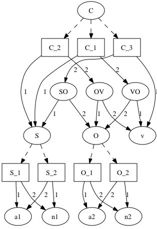
Figure 3: Plain forest of target-language trees that can correspond to the source-language tree inFigure 2.

We intersect/compose the packed forest with the bigram language modelΛby augmenting each node in the forest with a left context word and a right pe-ripheral word: a node N is transformed into a triple

(a,N,b) that dominates those trees which N domi-nates in the original forest and which can occur after a word a and end with a word b. The algorithm is roughly1as shown inFigure 5for binary branching forests; it requires memoization (not shown) to be efficient. The generalization to forests with arbitrary branching factors is straightforward, but the presen-tation of that algorithm less so. At the root level, we callforest_compositionwith a left context of # (indicating the start of the string) and add dummy nodes of the form(a,$,$)(indicating the end of the string). Further details can be found in the prototype implementation. Each node in the original forest is augmented with two words; if there are n leaf nodes in the original forest, the total number of nodes in the augmented forest will be at most n2times larger than in the original forest. This means that the com-pact encoding property of the packed forest (expo-nentially many trees can be represented in polyno-mial space) is preserved by the composition algo-rithm. An example of composing a packed forest

1_{A detailed implementation is available fromhttp://www.}

cs.columbia.edu/∼jansche/transfer/.

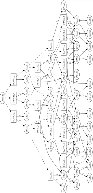
with a bigram language model appears inFigure 4, which shows the forest that results from composing the forest inFigure 3with a bigram language model. The result of the composition is an augmented forest from which sampling is almost trivial. The first thing we have to do is to recursively propagate weights from the leaves upwards to the root of the forest and associate them with nodes. In the non-recursive case of leaf nodes, their weights are pro-vided by the bigram score of the augmented forest: observe that leaves in the augmented forest have la-bels of the form(a,b,b), where a and b are terminal symbols, and a represents the immediately preced-ing left context. The score of such a leaf is sim-ply Λ(b|a). There are two recursive cases: For choice nodes (and-nodes), their weight is the prod-uct of the weights of the node’s children times a lo-cal likelihood score. For example, the node(v,O,n)

in Figure 4 dominates a single choice node (not shown, per the earlier conventions), whose weight is Λ(a|v)Λ(n|a)Ξ7. For other forest nodes (or-nodes), their weight is the sum of the weights of the node’s children (choice nodes).

prod-(# ,r o o t, $ ) (# ,r o o t, $ )_ 1 (# ,r o o t, $ )_ 2 (# ,r o o t, $ )_ 3 (# ,C ,n ) 1 (n ,$ ,$ ) 2 (# ,C ,n )_ 1 (# ,C ,n )_ 2 (# ,C ,n )_ 3 (# ,S ,n ) 1 (n ,V O ,n ) 2 (# ,a 1 ,a ) 1 (a ,n 1 ,n ) 2 (n ,v ,v ) 1 (v ,O ,n ) 2 (v ,a 2 ,a ) 1 (a ,n 2 ,n ) 2 (# ,S ,a ) 1 (a ,V O ,n ) 2 (# ,n 1 ,n ) 1 (n ,a 1 ,a ) 2 2 (a ,v ,v ) 1 (# ,v ,v ) 1 (v ,S O ,n ) 2 (v ,S O ,n )_ 1 (v ,S O ,n )_ 2 (v ,S ,n ) 1 (n ,O ,n ) 2 2 (v ,a 1 ,a ) 1 2 (n ,a 2 ,a ) 1 (v ,S ,a ) 1 (a ,O ,n ) 2 2 (v ,n 1 ,n ) 1 2 (a ,a 2 ,a ) 1 (# ,C ,a ) 1 (a ,$ ,$ ) 2 (# ,C ,a )_ 1 (# ,C ,a )_ 2 (# ,C ,a )_ 3 1 (a ,V O ,a ) 2

1 (v,O

,a ) 2 (v ,n 2 ,n ) 1 (n ,a 2 ,a ) 2 1 (n ,V O ,a ) 2 1 2 1 (v ,S O ,a ) 2 (v ,S O ,a )_ 1 (v ,S O ,a )_ 2 1 (a ,O ,a ) 2 2 (a ,n 2 ,n ) 1 1 (n ,O ,a ) 2 2 (n ,n 2 ,n ) 1 (# ,C ,v ) 1 (v ,$ ,$ ) 2 (# ,C ,v )_ 1 (# ,C ,v )_ 2 1 (n ,O V ,v ) 2 (n ,O V ,v )_ 1 (n ,O V ,v )_ 2 2 1 2 1 1 (a ,O V ,v ) 2 (a ,O V ,v )_ 1 (a ,O V ,v )_ 2 2 1 2 1

forest_composition(N, a): if N is a terminal:

return { (a,N,N) } else:

nodes = {}

for each (L,R) in N.choices:

left_nodes <- forest_composition(L, a) for each (a,L,b) in left_nodes:

right_nodes <- forest_composition(R, b) for each (b,R,c) in right_nodes:

new_n = (a,N,c)

nodes <- nodes + { new_n }

new_n.choices <- new_n.choices + [((a,L,b), (b,R,c))] return nodes

Figure 5: Algorithm for computing the intersection of a binary forest with a bigram language model.

uct of the local likelihood scores times the language model score of the tree’s terminal yield. We can then associate outgoing normalized weights with the children (choice points) of each or-node, where the probability of going to a particular choice node from a given or-node is equal to the weight of the choice node divided by the weight of the or-node.

This means we have managed to calculate the normalizing constant of the latent tree posterior(5)

without enumerating the individual trees in the for-est. Normalization ensures that we can sample from the augmented and normalized forest efficiently, by proceeding recursively in a top-down fashion, pick-ing a child of an or-node at random with probability proportional to the outgoing weight of that choice. It is easy to see (by a telescoping product argument) that by multiplying together the probabilities of each such choice we obtain the posterior probability of a latent tree. We thus have a method for sampling la-tent trees efficiently from their posterior distribution.

The sampling procedure described here is very similar to the lattice-based generation procedure with n-gram rescoring developed by Langkilde (2000), and is in fact based on the same intersection construction (Langkilde seems to be unaware that the CFG-intersection construction from (Bar-Hillel et al.,1961) is involved). However,Langkildeis in-terested in optimization (finding the best tree in the forest), which allows her to prune away less prob-able trees from the composed forest in a procedure

that combines composition, rescoring, and pruning. Alternatively, for a somewhat different but related formulation of the probability model, the sampling method developed byMark et al.(1992) can be used. However, its efficiency is not well understood.

5 Conclusions

The approach described in this paper was illustrated using very simple examples. The simplicity of the exposition should not obscure the full generality of our approach: it is applicable in the following situa-tions:

• A prior over latent trees is defined in terms of stochastic finite automata.

• The inverse image of an observed tree under the mapping from latent trees to observed trees can be expressed in terms of a finite context-free language, or equivalently, a packed forest.

The purpose of Gibbs sampling is to simulate the posterior distribution of the unobserved variables in the model. As the sampling procedure converges, knowledge contained in the informative but struc-turally weak priorΛis effectively passed to the syn-tactic transfer model Ξ. Once the sampling proce-dure has converged to a stationary distribution, we can run it for as many additional iterations as we want and sample the imputed target-language trees. Those trees can then be collected in a treebank, thus creating novel syntactically annotated data in the tar-get language, which can be used for further process-ing in syntax-based NLP tasks.

Acknowledgements

I would like to thank Steven Abney, the participants of the 2005 Johns Hopkins workshop on Arabic di-alect parsing, and the anonymous reviewers for help-ful discussions. The usual disclaimers apply.

References

Y. Bar-Hillel, M. Perles, and E. Shamir. 1961. On formal properties of simple phrase structure grammars. Zeitschrift f¨ur Phonetik, Sprach-wissenschaft und Kommunikationsforschung, 14(2):143–172.

Alan E. Gelfand and Adrian F. M. Smith. 1990. Sampling-based approaches to calculating marginal densities. Journal of the American Statistical Association, 85(410):398–409.

Stuart Geman and Donald Geman. 1984. Stochastic relaxation, Gibbs distributions, and the Bayesian restoration of images. IEEE Transactions on Pattern Matching and Machine Intelligence, 6(6):721–741.

Irene Langkilde. 2000. Forest-based statistical sentence generation. In Proceedings of the First Meeting of the North American Chapter of the Association for Computational Linguistics, pages 170–177. ACL Anthology A00-2023.

Jun S. Liu. 2001. Monte Carlo Strategies in Scien-tific Computing. Springer.

Mohamed Maamouri, Ann Bies, Tim Buckwalter, and Hubert Jin. 2004a. Arabic Treebank: Part 2 v 2.0. Electronic resource, available from LDC.

Mohamed Maamouri, Ann Bies, Tim Buckwalter, and Hubert Jin. 2004b. Arabic Treebank: Part 3 v 1.0. Electronic resource, available from LDC.

Mohamed Maamouri, Ann Bies, Hubert Jin, and Tim Buckwalter. 2003. Arabic Treebank: Part 1 v 2.0. Electronic resource, available from LDC.

Kevin Mark, Michael Miller, Ulf Grenander, and Steve Abney. 1992. Parameter estimation for constrained context-free language models. In Speech and Natural Language: Proceedings of a Workshop Held at Harriman, New York, Febru-ary 23–26, 1992, pages 146–149. ACL Anthol-ogy H92-1028.

Martin A. Tanner and Wing Hung Wong. 1987. The calculation of posterior distributions by data aug-mentation. Journal of the American Statistical Association, 82(398):528–540.