Value at Risk:
Applications for Analysis and Disclosure in the U.S. Banking Sector
July 2001
Abstract
The purpose of this paper is to encourage banks to extend existing market risk management analysis and disclosure via the well-known Value-at-Risk (VaR) methodology. An extension from trading book VaR to structural VaR is developed. In addition to the standard benefits of VaR measurement, two lesser-known benefits of the VaR process are highlighted:
ï Efficient selection of portfolio-specific "worst case" stress test; and ï Determination of directionality in interest rate risk management
In order to help equity analysts and investors better understand the market risk tradeoffs inherent in banking the efficacy of disclosing Earnings-at-Risk (EaR) measures in conjunction with VaR is discussed.
Market Risk Reporting Requirements
The Securities and Exchange Commission (SEC) requires reporting banks to disclose quantitative and qualitative information about market risk (SEC, 1997). Three disclosure formats are suggested:
ï Tabular presentation of future cash flows with related fair values. This usually takes the
form of a liquidity GAP table (circa 1980) and Fair Value disclosures proscribed by SFAS 107 (circa 1990).
ï A sensitivity analysis disclosing earnings, cash flows, or value changes based on
hypothetical rate changes (e.g. +/- 100, 200, 300 basis points). This format is similar to the requirements of Thrift Bulletin 13, promulgated in 1987.
ï A probabilistic Value at Risk (VaR) analysis disclosing earning, cash flow, or value
changes emanating from market movements.
Compliance among the very largest financial firms has been quite high (Blankley, 2000). At non-bank financial firms, this has evolved into the generalized use of VaR disclosures. Within the banking sector, at the largest of banks, the VaR disclosure is typically used only for the trading book, comprising a small portion of assets. Most banks disclose their market risk positions using the cash flow or sensitivity measures, based on static or deterministic interest rate scenarios.
Table 1
VaR Profile by Risk Type: 2000 In millions
Risk Category High Low Average Interest Rate 15.3 1.2 8.9 Foreign Exchange 3.3 0.3 1.3
Equity 7.8 0.3 4.0
Aggregate 15.5 5.5 10.2
This probabilistic disclosure, infrequent as is it in the banking sector, deals only with the trading book of the bank, comprising approximately 5% of assets. The remaining 95% of assets, all liabilities, and capital are ignored in this VaR disclosure. The remainder of the bank, or the structural bank, as it is commonly referred to, is covered in the less rigorous sensitivity analysis disclosure format utilizing deterministically based, implausible parallel yield curve shifts. Prior to reviewing our structural VaR approach, a brief review of VaR methodology is presented.
VaR Methodologies
As is well known, there are three primary VaR calculation methodologies:
1) Parametric methods variously referred to as the correlation-covariance method, or the delta-normal or delta–gamma approaches. J.P. Morgan standardized this as RiskMetrics in 1994. This is typically a closed-form process and is used by some financial firms to analyze and disclose market risk.
2) Historical simulation, or extreme event stress tests. This methodology replicates market risk factors including:
ï The 1987 U.S. equities market crash.
o 1994, when the Fed Funds rate increased 250 basis points.
o 1977-1981, when the Fed Funds rate increased over 1500 basis points in forty-eight months.
ï Rapid interest rate decreases, in the following years:
o 2001, when the Feds Fund rate decreased by 250 basis points in six months.
o 1991-93, when the Fed Funds rate decreased 500 basis points in twenty-four months.
3) Monte Carlo or Quasi- Monte Carlo methods, perhaps more correctly a stochastic process. At its simplest, Monte Carlo simulation is the procedure by which random future rate paths are generated and used to derive path dependent cash flow schedules. It uses stochastically generated rate paths and associates cash flows to value interest rate contingent financial instruments (Linsmeier, 2000 and Rahl, 2000).
VaR Benefits
Given the relatively large resource commitment to implementing a VaR process, it is doubtful that financial institutions utilize their VaR-based risk analyses and reporting solely for regulatory compliance. Rather the implementation of a VaR-based market risk system has significant benefits, with regulatory compliance an ancillary benefit. These include:
ï A way to describe the magnitude of likely losses in a portfolio. ï The likelihood of those losses.
Stakeholders in publicly traded banks should favor and benefit from the increased risk- management capabilities that the VaR process provides, as well as their disclosure.
Market Risk Analysis for the Structural Bank Balance Sheet
Most VaR-based market risk disclosures utilize a VaR process based on closed-form solutions and focus on the very short-term, usually one to thirty days. In the banking sector, market risk disclosures utilize an opposite, and perhaps apposite approach, focusing on the effective lives of assets and liabilities utilizing simulation analysis. In addition, banking market risk disclosures tend to focus solely on the interest rate risk component of market risk, as does this article. Note that this approach can be readily extended for joint or separate consideration of credit, liquidity and other risk types (Bangia, 1998 and Ho, 1999).
Trading portfolio assets tend to have well-defined cash flow characteristics, with standardized cash flow mapping, and readily available correlations and cross-correlations. Bank balance sheets, in comparison, are replete with financial instruments with either indeterminate and/or interest rate contingent cash flows. More intricate examples include credit card and line of credit loan types, also seen in investment portfolios in securitized equivalents and non-maturity deposits. Due to the predominance of option-laden instruments on bank balance sheets, closed-form solutions are not typically used for the structural bank, except in stylized examples (Ho, 1999).
public, secondary marketplaces, industry-standard valuation approaches (e.g. Discounted Cash Flow, Option Adjusted Spread and matrix pricing, etc.) are utilized. Modeling and valuing structural balance sheets can be problematic, as one class of financial instruments, non-maturity deposits (e.g. demand, savings, and money market deposit types) comprise up to fifty percent of bank liabilities. Lacking a public market, there is no general consensus regarding appropriate modeling and valuation methodologies among marketplace participants, regulators and academia for non-maturity deposits.
Partial details of the approach utilized by the author to value non-maturity deposits have been presented elsewhere, but the full explication is in pre-publication status (Poorman, 2000 and 2001-2). A relevant analogy to our proprietary method would be to refer to Bloomberg Financial’s use of prepayment estimates from various models and methodologies to develop a median market consensus estimate (Hayr, 2000). In general, it is worth noting that most observers agree that bank non-maturity deposits exhibit sticky, asymmetric behavior pricing behaviors, while disagreeing on standard financial instrument metrics including duration, fair value, and sensitivity to interest rate changes (Hawkins, 2000 and Poorman, 2001-2).
Within the banking sector, the primary method for analyzing and managing market risk is usually referred to as Asset/Liability Management (A/LM). A/LM has been defined as: “The coordinated approach to the management of loans, investments, deposits, borrowing, capital, and liquidity in order to achieve the institution’s objectives within prudent risk limits (Essert, 1997).” The goal of successful A/LM is seen as “ensuring that net interest income and the net economic value of the balance sheet remain positive and stable under all probable scenarios (Essert, 1997)”. Correspondingly, bank market risk models are frequently referred to as A/LM models.
Some of the more advanced vendor-built A/LM models used by the banking sector are capable of producing VaR analyses utilizing historical and/or stochastic process approaches. A necessary and integral component of a VaR-based bank A/LM approach is a suitable interest rate model. Minimum requirements for utilization of a stochastic interest rate model include:
ï Creation of arbitrage-free forward term structures of interest rates. ï Capability of utilizing historical or implied market volatilities.
Numerous interest rate models have been proposed for evaluating rate-contingent financial instruments. The model used and discussed herein is the well-known continuous single factor Black-Derman-Toy (B-D-T) model (Black, 1990). In this VaR analysis, the B-D-T model is modified for user-defined selection of:
ï Long volatility; ï Short volatility; and
The strengths and limitations of the B-D-T model are well known, which is of benefit to marketplace participants (Kazziha, 1997). As such, the B-D-T model is commonly used to model fixed income securities and derivatives. For example, it is used in Bloomberg Financial’s Option Adjusted Spread (OAS) analysis to benchmark fixed-income values, including those derived via bank A/LM models.
The selection of a stochastic rate component is equally important in generating and valuing rate-contingent cash flows (Payant, 1995). The primary choices include:
ï A random Monte Carlo simulator; or ï A lattice based model, primarily:
o Binomial (rates go up or down), or
o Trinomial (rates go up, down, or remain stationary).
The sampling reduction is important as computation time, and resultant analytical time, are non-trivial, as a 360-month binomial lattice has 2360 interest rate paths. The sampled linear path space represents 89.9% of the 2360 paths, reduced to a more manageable, and probability-ranked, 269 paths. Further, the implementation reviewed herein uses 101 of the highest probability LPS paths, which is equivalent to 91.3% of the linear path space, and is in excess of 80% (89.9 x 91.3) of the 2360 binomial lattice. This reduction approach is congruent with the notion of Pareto optimization, known as “the 80/20 rule in A/LM” (Uyemura, 1993).
Suggested VaR Disclosure Format
At a minimum, our suggested disclosure format follows the abbreviated example of Table 1, but includes the entire balance sheet and uses the “lifetime VaR”, rather short-term VaR (Arnold, 1998). The suggested format also uses percentages of EVE at risk, congruent with regulatory and industry practice used for the sensitivity disclosure format (FFIEC, 1997). Our examples utilize two banks scaled to a common size ($20 billion assets), with balance sheets, interest rates and implied swaption volatilities as of March 2001.
A sample market risk disclosure should read: Our lifetime VaR limit for the Economic Value of Equity is 25% … we calculate lifetime VaR… at the 99% confidence level (two tailed).
Table 2
VaR Profile: March, 2001
Next, add a more complete VaR profile for internal reporting, and possibly for external disclosure purposes, including at a minimum:
ï Tabular, or numerical descriptions of the probability distributions; and ï Graphical depictions of the same.
Chart 1
VaR Profile: March, 2001 $ 000
A fuller set of probabilistic disclosures allows for a more comprehensive analysis of the VaR profile, including skewness and kurtosis. In the example above, the outcomes are skewed to the left or toward unfavorable results, consistent with the negative convexity of many bank assets and leveraged balance sheets. Disclosure of this profile would allow investors to more carefully select suitable bank equity investments, based on their individual utility functions, as expressed by risk/return preferences.
0% 25% 50% 75% 100%
2,323,329 2,479,811 2,636,294 2,792,776 2,949,258 3,105,740 3,262,223 3,418,705 Probability
Cumulative Probability
Standard deviations <-3 -3 to -2 -2 to -1 -1 to mean mean to +1 +1 to +2 +2 to +3 +3 to +4 Market Value 2,323,329 2,479,811 2,636,294 2,792,776 2,949,258 3,105,740 3,262,223 3,418,705
Probability 1% 4% 13% 18% 46% 18% 0% 0%
In the banking sector, it is customary to refer to a bank’s market risk exposure to interest rates by referring to them as either asset- or liability-sensitive. This shorthand jargon emanates from the use of GAP analysis and disclosure in the early 1980s; nonetheless, it is still commonplace. The so-called asset-sensitive bank benefits from increasing rates, whereas the liability-sensitive bank benefits from decreasing rates. An indication of directional exposure to interest rate changes is the focus of the sensitivity analysis disclosure format, but this is frequently excluded from VaR disclosures. Therefore, supplemental analysis and disclosure may be useful to the investing public:
ï A measure of directionality; ï A valuation benchmark; and
ï The goodness of fit, or R2, of the measure.
Chart 2
VaR Profile: March, 2001 $000
In this VaR construct, the use of volatility shocks, or alternative volatility scenarios, may serve as another variant of stress testing. Combined with goal-seeking methodologies, subject to real world constraints, the VaR toolkit may be expanded to include value optimization for the structural bank.
Earnings-at-Risk (EaR) measures
Although VaR has received much academic and marketplace attention, it is arguable that both bank managements and investors remain focused on earnings-based approaches. The use of VaR and EaR disclosures is not an either/or proposition, rather it is, or should be, an “and” proposition. Our EaR analysis and sample disclosures use the same format and bank previously used for the VaR analysis. A sample EaR disclosure should read: Our first year EaR limit for Net Interest Income (NII) is 10% … we calculate first year EaR … at the 99% confidence level.
Economic Value of Equity
2,000,000 2,250,000 2,500,000 2,750,000 3,000,000 3,250,000
Table 3
EaR Profile: March, 2001
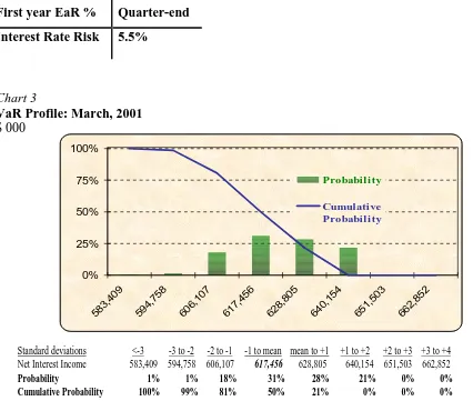
First year EaR % Quarter-end Interest Rate Risk 5.5%
Chart 3
VaR Profile: March, 2001 $ 000
A fuller set of probabilistic disclosures allows for a more comprehensive analysis of the EaR profile, including skewness and kurtosis. In the example above, the outcomes are somewhat normally distributed, with slight kurtosis. Disclosure of this EaR profile, in conjunction with the VaR profile, would further allow investors to select suitable equity investments, based on their individual utility functions. As with the VaR disclosure, an EaR disclosure indicating directional sensitivity should be included.
Chart 4
VaR Profile: March, 2001 $000
The above example uses the average (earnings horizon) one-year swap rate as a benchmark. A simple linear regression of the benchmark rate, or key duration, versus EVE suggests that there is a strong linear relationship between variables, with an unadjusted R2 = 0.9416. It may be of interest to note that the most negative outcome is based on the most extreme increasing rate scenario (identified by the color-coded data point). The same scenario that results in the most unfavorable long-term results, as measured by VaR, results in the “worst case” scenario from an earnings standpoint. Several points are worth highlighting:
ï A short-term rate decrease is favorable from an earnings and a valuation standpoint. Note
that this is not necessarily always the case
ï The selection of risk mitigation strategies, including off-balance sheet hedging may be
dependent on income/value tradeoffs.
ï Different benchmarks, or key rates, may be significant for value and earnings measures,
Net Interest Income
Comparative Analysis and Investor Utility
Bank A, in isolation, provides a case study for structural VaR and EaR analysis and disclosure. Investment decisions, including stock selection, are usually not made in isolation without consideration of inter- and intra-sector alternatives. Many, especially so-called active investors and managers, believe that security selection, rather than sector- or asset class-allocation, is the primary performance determinant. It is only by comparison to investment alternatives that utility preferences, or unique risk/return profiles are established. To establish the utility preference hierarchy, or the “optimal frontier,” the VaR and EaR profiles of Banks A and B are presented (Schirripa, 2000).
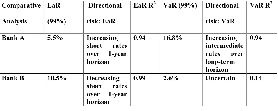
Table 4
EaR & VaR Profiles: March, 2001
With disclosure of EaR and VaR measures, including interest rate directional exposure, investors can select suitable investments based on their risk preferences and views on prospective interest rate changes. In the context of utility and optimal frontier theory:
ï Investors preferring less VaR volatility would prefer Bank B to Bank A.
ï Short-term, earnings-focused investors with a bias towards continued decreases in short
rates would, ceteris paribus, prefer Bank A to Bank B.
References
Arnold, Michael, “Hedging Interest Rate Risk from Both an Economic Value and Earnings Perspective”, San Francisco GARP Presentation, 1998.
Bangia, A., F. Diebold, T. Schuermann, and J. Stroughair, “Modeling Liquidity Risk, With Implications for Traditional Market Risk Measurement and Management, Wharton Financial Institutions Center, 1998.
Black, Fischer, Emmanuel Derman and William Toy, “A One-Factor Model of Interest Rates and Its Application to Treasury Bond Options”, Financial Analysts Journal, 1990.
Blankley, Alan, Reinhold Lamb, and Richard Schroeder, "Compliance with SEC Disclosure Requirements About Market Risk," Journal of Derivatives, Spring 2000.
Breuer, Thomas and Gerald Krenn, “Identifying Stress Test Scenarios”, Fachhoochshule Voralberg and Oesterreichische Nationalbank, respectively, 2000.
Essert, James, “Asset/Liability Management 101”, Sendero Institute presentation, 1997.
FFIEC Uniform Financial Institutions Rating System, 1996.
First Union Corp., 2001 Annual Report.
Hawkins, Raymond and Michael Arnold, “Relaxation Processes in Administered-Rate Pricing”, Physical Review, 2000.
Ho, Thomas, “Key Rate Durations: Measures of Interest Rate Risks”, Journal of Fixed Income, September 1992.
Ho, Thomas, “Managing Illiquid Bonds and Linear Path Space”, Journal of Fixed Income, June 1992.
Ho, Thomas, Mark Abbott, and Allen Abrahamson, “Value at Risk of a Bank’s Balance Sheet”, International Journal of Theoretical and Applied Finance, 1999.
Kazziha, Soraya and Riccardo Rebanato, “Unconditional Variance, Mean Reversion and Short Rate Volatility in the Calibration of the Black-Derman and Toy Model and of Two-Dimensional Log-Normal Short Rate Models, Net Exposure, November 1997.
Linsmeier, Thomas J. and Neil D. Pearson, "Value At Risk," Financial Analysts Journal, March/April, 2000.
Payant, Randall, "Go with the Flow," Balance Sheet, Spring 1995.
Poorman, Jr., Fred, “An Overview of Core Deposits”, Bank Asset/Liability Management, 2000.
Poorman, Jr., Fred, “Valuing Core Deposits”, Bank Accounting & Finance, publication pending, Winter 2001-2.
SEC: Disclosure Of Accounting Policies For Derivative Financial Instruments And Derivative Commodity Instruments And Disclosure Of Quantitative And Qualitative Information About Market Risk Inherent In, Derivative Financial Instruments, Other Financial Instruments And Derivative Commodity Instruments, 1997.
Uyemura, Dennis and Donald Devanter, “Financial Risk Management In Banking”, Bankers Publishing Company, 1993.